First steps in R

1 Get ready for the course

Before the course starts, you should have installed R and RStudio on your computer (see below). RStudio is highly recommended, especially if you are a beginner.

1.1 About R

This course will use a programming language oriented towards data analysis and statistics: R.

It can be useful for:

• Publication ready graphs
• Biological analysis libraries
• Statistical testing
• Many more: table reformatting, maps, interactive visualizations, etc…

R can be used in an interactive console: typing and executing commands one by one.

Another way to work with R is to prepare a list of commands in a text file (a script, which is a kind of program) and then tell R to execute them. This is an excellent way to have reproducible and well documented analyses.

1.2 About RStudio

RStudio is an application in which you can load data, execute R commands, prepare scripts, get information on commands and environments (the current state of your work), visualize graphics and more.

You do not need RStudio to work with R, but it will make your life easier during this course.

1.3 Installing R

R can be obtained from the following site: https://cran.rstudio.com/

Try to install version 3.5 or above (and preferably at least 3.6). If your operating system provides R already, but in a slightly earlier version, most things in the present course will probably work fine, but this might not be true for later R-based courses, and you will run into trouble sooner or later.

• For those using a Debian or Ubuntu based Linux, we suggest reading the following material before proceeding to install R: https://github.com/blaiseli/R_install_notes/blob/master/Install_Linux.md. Some of the content may also be helpful for users of other types of Linux distributions.

• Windows users should refer to the following page: https://cran.rstudio.com/bin/windows/base/

• Mac OSX users should refer to this one: https://cran.rstudio.com/bin/macosx/

1.4 Installing RStudio

You can obtain RStudio from this page: https://www.rstudio.com/products/rstudio/download/

• Choose the free version (“RStudio Desktop, Open Source Licence”).

• Download and run the “installer” suitable for your operating system.

1.5 Course material

• The most up-to-date version of the present course support should be available at http://hub-courses.pages.pasteur.fr/R_pasteur_phd/First_steps_RStudio.html
• If you spot typos, errors, ambiguities, etc., you can sign in on our local gitlab server using your Pasteur ID (if you are a member of the Institut Pasteur) or using a github account to submit an issue here: https://gitlab.pasteur.fr/hub-courses/R_pasteur_phd/issues
• You can get the full course material (html page, data for the exercises, and more) in the following zipped archive (recommended): http://hub-courses.pages.pasteur.fr/R_pasteur_phd/2020-03/First_steps_RStudio.zip

The course contains small exercises (indicated with ) to help you memorize the techniques we present. Try to search by yourself, then discuss with your neighbours (if you want), before clicking on the “Hint” buttons. There are often several ways to solve a problem when programming. If you come up with solutions other than the ones we propose, while still using techniques already seen in the course, don’t hesitate to share them with us.

The buttons with the icon open sections that will not be treated during the course. Feel free to study them when you have free time (if the course pace is too slow for you, for instance).

Here’s one already!

Recompiling the html page

In the full course archive, you will find the Rmarkdown source (.Rmd) from which the html page is automatically generated.

You can open it in RStudio.

You can then re-create the html page using the “Knit” () button.

(This will fail if the images and data directories are not present in the same folder as the Rmarkdown file.)

This allows you to add your own notes and experiments with R in the .Rmd file, and create your own personalized version of the course (don’t waste too much time playing with this during the course).

For those working on Linux:

# Download the archive:
wget http://hub-courses.pages.pasteur.fr/R_pasteur_phd/2020-03/First_steps_RStudio.zip
# Extract it:
unzip First_steps_RStudio.zip
# Go in the extracted directory:
cd First_steps_RStudio
# Optionally:
# Edit the .Rmd file with RStudio or your favourite text editor
# Recompile the html document (without even needing to use RStudio!):
make
# Open the local html file (with firefox, for instance):
firefox First_steps_RStudio.html

The above might work on Mac OSX too (not tested).

The material for the other modules of the course is (or will soon be) available at https://c3bi.pasteur.fr/bioinformatics-program-for-phd-students-2019-2020/.

2 Smooth introduction to R

2.1 The RStudio interface

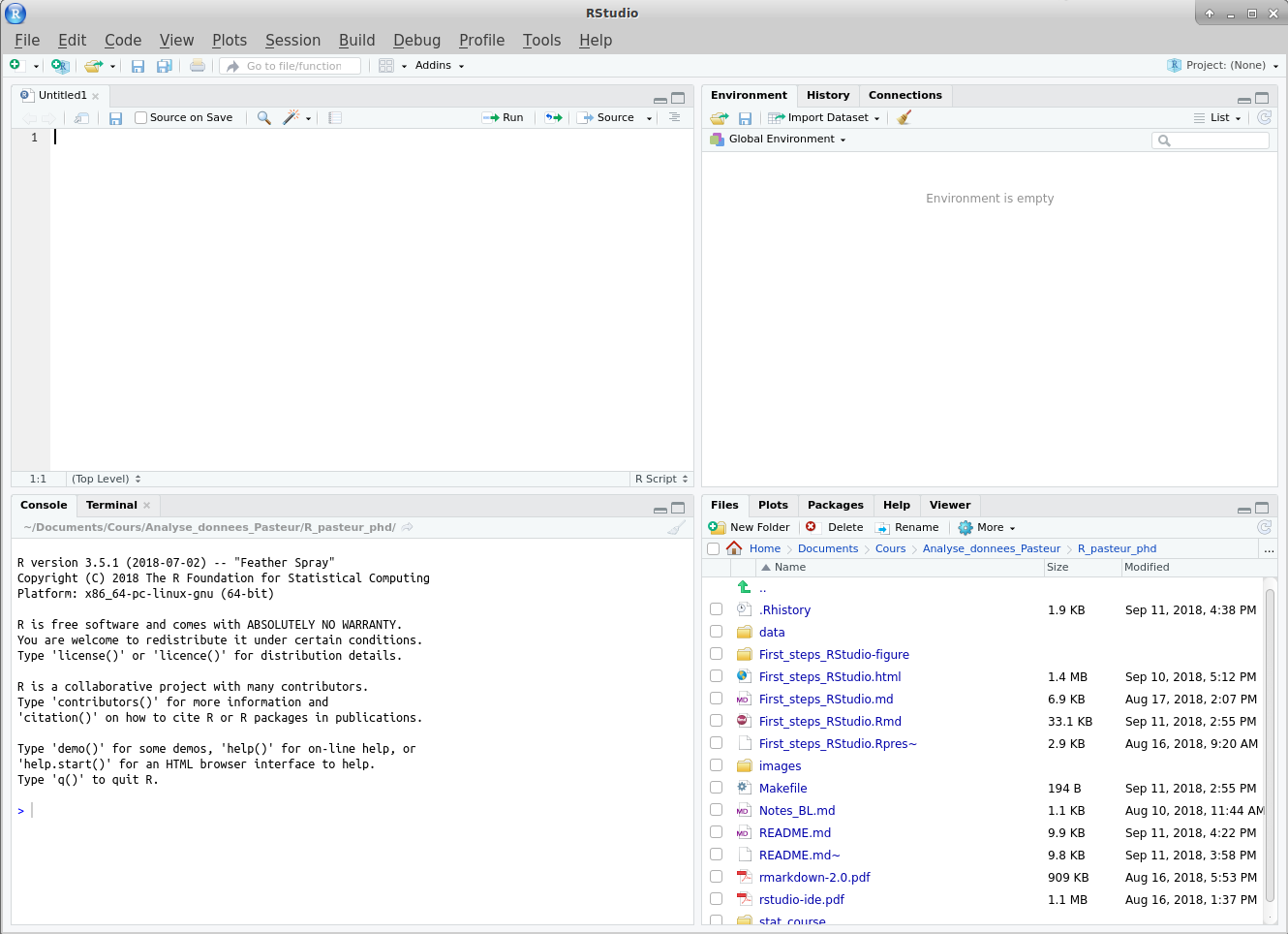
By default, RStudio opens with three or four panes, each containing several tabs:

• The top-left pane (if present, otherwise click ) is the editor, where you can write scripts, and other types of documents. This is also where data frames can be visualized.
• The bottom-left one contains the “Console”, where you can directly type R commands.
• The top-right one contains information about the “Environment”: values currently defined in your R session.
• The bottom-right one contains various tabs, including the following ones:
  • a file explorer
  • a help viewer
  • a plot visualizer
  • a package manager (packages are a way to extend the functionalities of R).

2.2 Loading data in RStudio

A frequent use of R is to analyse data stored as tables in files.

2.2.1 Quick dive in Milieu Intérieur dataset

The “Milieu Intérieur” project is an ambitious population-based study coordinated by the Institut Pasteur, Paris. The objective is to dissect the interplay between genetics and environment and their impact on the immune system (https://research.pasteur.fr/en/program_project/milieu-interieur-labex/).

More on Milieu Intérieur

This project is named after the French physiologist Claude Bernard’s concept of milieu intérieur and aims to establish the determinants of a healthy immune response by identifying genetic and environmental factors that contribute to the observed heterogeneity of immune responses. Restoring the “personal” in medical care is a major challenge for medicine, and the driving vision of the project. This project is coordinated by Pr Matthew Albert and Dr Lluis Quintana-Murci and is part of a larger French Governmental Initiative called Investissement d’Avenir – Laboratoire d’Excellence (LabEx).

Download the Milieu Intérieur dataset from http://hub-courses.pages.pasteur.fr/R_pasteur_phd/data/mi.csv, and remember where in your computer it was saved.

The “Environment” tab of the top-right pane of RStudio contains an “Import Dataset” button () that can be used to load various kind of files.

Open the “Import Dataset” menu and choose “From Text (base)…”.

A file browser will open. Select the file you just downloaded.

You should see a window presenting you options related to how the content of the file should be interpreted, similar to the following:

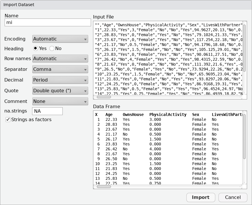
Most default values should be OK. Be sure that the “Heading” option is set to “Yes” and select “Use first column” for the “Row names” option, then click on the “Import” button.

A tab should open in the top-left pane displaying the content of the file. These data represent information pertaining to individuals that participated to the “Milieu Intérieur” study. Lines correspond to individuals (“observations”), and columns to various pieces of information obtained for them (“variables”).

In the “Environment” tab of the top-right pane of RStudio, you have access to more information about this table:

• next to the name of the table (mi, if you used the default choice at import), the number of observations and variables in the table;
• below (if you click on the arrow next to the name of the table), a listing describing how the data for each column is represented in R.

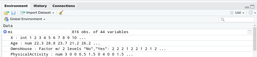
You can see that the information consists in numerical and textual information.

What we obtained by loading this file is called a “data frame” in R. A lot of things can be done using data frames, and we’ll learn some of it later in this course.

Briefly, and to wet your appetite, a specific column of a data frame can be accessed by using the name of the data frame (here mi), a dollar sign $ and the name of the desired column (here for example Age):

mi$Age

 [1] 22.33 28.83 23.67 21.17 26.17 23.83 26.42 21.67 26.50 23.25
 [ reached getOption("max.print") -- omitted 806 entries ]

You want to visualize the age distribution of this dataset ? To plot a histogram, just use the hist function:

hist(mi$Age)

A function is a predefined set of computations that can be re-executed, possibly with variations, depending on its arguments (the things given between the parentheses). Pre-defined functions, like hist help make R very useful for non-programmers.

But we are getting ahead of ourselves and we will see more on functions, data frames manipulation and data visualization later on\(\dots\) Before being able to actually analyse data, we will have to learn about the various ways used to represent data in R, and what kind of things can be done with data on a basic level.

2.3 R as a calculator

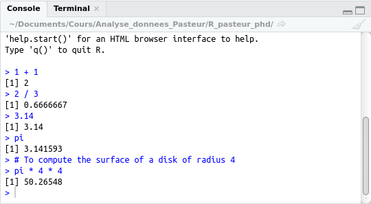
In the “Console” part of RStudio, you can see a prompt: This > symbol invites you to type commands.

Try the following (validate using the “return” key after typing):

> 1 + 1

[1] 2

It seems R gave the correct result (ignore the [1] for now).

Note that some complicated calculations may take a non-negligible time. A button should be visible until the calculation ends. If you suspect something is going wrong, use it to interrupt the calculation.

Once R is ready to take new commands, you should see a prompt (>) again in the console.

You can of course also subtract (-), multiply (*) and divide (/). Feel free to experiment with the usual mathematical operators.

2.4 Numbers

Divisions may give answers with a dot as decimal separator:

> 2 / 3

[1] 0.6666667

The result can be rounded for the display. The actual value may also sometimes not be mathematically exact. This is due to limitations inherent to the way numbers are encoded by the computer.

Use a dot, not a comma when writing numbers with decimals (called double in R):

> 3.14

[1] 3.14

By the way, R knows about \(\pi\):

> pi

[1] 3.141593

Scientific notation is allowed, and could be useful:

> 5e-3

[1] 0.005

Quotient and remainder

It is sometimes useful to compute quotients and remainders. This can be done using the integer division (%/%) and modulus (%%) operators:

> 5 %/% 2

[1] 2

> 5 %% 2

[1] 1

Computing the modulus 2 of a number is a common trick to determine whether it is even (the result is 0) or odd (the result is 1). More generally, when the modulus n of a number is 0, it means that this number is a multiple of n.

2.5 Variables

2.5.1 Defining and using variables

Like the predefined pi, you can temporarily “save” values in the computer memory by associating them to a name:

> my_variable <- 2 + 2

Some people tend to use the equal sign (=) instead of the above left-pointing arrow (<-). Both work in R.

Assignment

Many programming languages use the equal sign to do this kind of assignment. Assignment is almost always done with the value to assign on the right (“r-value”), and where to store it on the left (“l-value”). One peculiarity of R is that it also provides a way to assign the other way round, using a right-pointing arrow:

> 5 + 2 -> another_variable

The leftward assignment is so widespread in programming, that many people consider the above confusing.

You can then use the corresponding value by simply typing the associated name:

> my_variable

[1] 4

> my_variable * 5

[1] 20

This is called a variable: the associated value can be updated by later commands:

> my_variable <- 5
> my_variable

[1] 5

> my_variable <- 3
> my_variable

[1] 3

> my_variable <- 2 * 3
> my_variable

[1] 6

By the way, you can re-use the previous commands in the console by navigating the “command history” using the up and down arrows of your keyboard. You can then modify the selected command if needed (use the left and right arrows to get to the part you want to edit).

Note that the older values are now lost (variables are also lost when you quit or restart R).

You will use variables a lot. You can use them to store many different types of values that we will see later. For instance, the “Milieu Intérieur” data frame we previously loaded from a file is stored using a variable named mi.

Note that this notion of “variable” (in the “computer programming” sense) is not exactly the same as the one we used when referring to columns in the data frame, which is more a notion belonging to the data science field.

You can even store functions (sequences of commands that can be re-used).

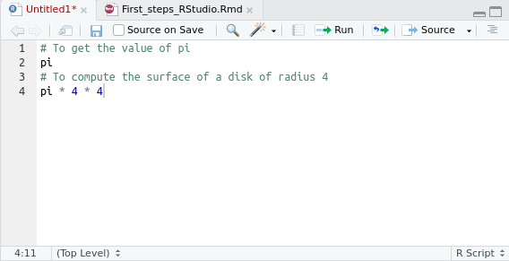
You can use a variable as many times as you wish in a calculation, and you can even use it to create another variable:

> radius <- 4
> area <- pi * radius * radius
> area

[1] 50.26548

Another handy feature provided by RStudio is code completion. You will notice it after typing three characters: a pop-up will appear giving you the variables and functions starting with these characters and available in the current environment. This pop-up is giving you a brief description as well. You can make the code completion pop-up also appear by pressing the TAB key (the one with a kind of arrow, located at the left of the first row of letters of most computer keyboards).

You can also see the variables you defined and their current value in the “Environment” tab (top-right pane).

2.5.2 Variable naming rules

Variable names need to conform to certain rules. You should be relatively safe if you stick to the following:

• Use only:
  • plain ASCII letters (“A” to “Z” and “a” to “z”);
  • numbers;
  • underscore ("_").
• Don’t start a variable name with underscore or a number.
• Avoid single letter unless meaning is obvious.
• Avoid using names that already exist (that’s the tricky part).

This is OK:

> five_point_6 <- 5.6

This is not (try it, you will get an error):

> 6_times_4 <- 24

## Error: <text>:1:2: unexpected input
1: 6_
     ^

You can do this, but you shouldn’t:

> pi <- 3.14

If you did it nonetheless (you fool…) the older and more accurate value of pi is still available as base::pi.

Reserved words

If you type ?Reserved in the R console, the “Help” tab of the bottom-right pane will give you a list of names that you really cannot use for your variables.

> Inf <- 999999999

## Error: invalid (do_set) left-hand side to assignment

The names of your variables should help you and others understand what the code is supposed to do.

You will sometimes see dots (.) in variable names. This is allowed in R, but in many programming languages, dots have special meanings. You’d better avoid taking the habit of using dots in variable names. This will make the transition less painful if you ever decide to learn other languages.

2.6 Intermission: Scripts in RStudio

2.6.1 Getting organized

Above the console, there is a space where you can take note of the commands you want to remember, and save this to a (plain text) file.

This is actually intended to create a script. A script is a file containing a succession of commands that can be executed to do all the corresponding computations. Just put a # before the parts that are not valid R commands.

This is called “commenting”, and it is a good practice to put such comments in your scripts, especially in parts that took you time to get right. That helps you remember what your intentions were when you wrote the commands (and can also help others, if you share your scripts).

(You can use the button to create a new script or in the menu “File” > “New File” > “R Script”.)

Small script example:

2.6.2 Executing saved scripts

• Execute code on the current line (or block of selected lines) in the console below (shortcut: (Ctrl or Cmd) + Enter).
• Execute the whole script in the console below (shortcut: (Ctrl or Cmd) + Shift + Enter).

(You can also execute an R script outside RStudio, using the Rscript command from a command line interface.)

Example of execution of the current line:

(The preceding comments have also been “executed”: they appear in the console, but have no other effects.)

2.7 Truth values (“Booleans”)

You can compare numbers using comparison operators:

3 * 2 > 4

[1] TRUE

1 <= -3

[1] FALSE

Double equal == is used to test equality:

5 == 2 + 3

[1] TRUE

!= (not equal) is used to test inequality:

1 + 3 != 4

[1] FALSE

The result of a comparison is a value that tells you whether what you wrote is true or not. Such values are called Boolean values, or “Booleans” (after the logician George Boole).

They must be written in capitals:

TRUE

[1] TRUE

FALSE

[1] FALSE

Otherwise, R looks for a variable with that name:

true

## Error: object 'true' not found

Don’t name your variables with names such as true or false, you might get bitten.

Code failing with an error message is often better than undetected mistakes.

2.7.1 Boolean operations

You can use Booleans to compute more Booleans, using logical operators:

TRUE & FALSE  # And

[1] FALSE

TRUE | FALSE  # Or

[1] TRUE

!FALSE  # Not

[1] TRUE

FALSE & ((1 == 1) | TRUE)

[1] FALSE

In the last command, we mix comparison expressions (that have Boolean results) with “literal” Booleans (FALSE and TRUE) The whole result has a Boolean value.

Expressions can be composed of a hierarchy of expressions combined with operators. Operators have precedence rules, telling what operations should be evaluated first.

To be sure that expressions will be evaluated in the intended order, we can use parentheses in complex expressions, as above. Here is a decomposition of the evaluation:

• 1 == 1 is TRUE, therefore ((1 == 1) | TRUE) is TRUE.
• This expression is hence equivalent to FALSE & TRUE, which is FALSE.

(Parentheses can be used in any expression, not just in Boolean calculations.)

2.8 Strings (text)

Computer programs are much more useful for humans if they can communicate with them using text, and let them manipulate text, and not just simple mathematical objects such as numbers or Booleans. Indeed, text is a powerful tool to convey complex information. Text can be used to encode information in various ways.

Fortunately, R offers (and heavily uses) the possibility to represent text.

We can define character strings (or just “strings”) variables to represent text, placing it "between quotes":

selected_color <- "blue"
file_name <- "counts.csv"

Note that there are no quotes when one writes TRUE, FALSE or a variable name. This is a very important difference to keep in mind.

We will see later what can be done with strings.

3 Vectors

3.1 Creating or getting vectors

You can group values of the same type in a vector, using c (combine).

Numbers:

my_numbers <- c(6, -1, 0, 6)
my_numbers

[1]  6 -1  0  6

Strings:

phenotype <- c("round", "wrinkled", "round", "wrinkled")
phenotype

[1] "round"    "wrinkled" "round"    "wrinkled"

Booleans:

tests <- c(TRUE, FALSE, FALSE, TRUE)
tests

[1]  TRUE FALSE FALSE  TRUE

Of course, values in a vector can be the result of a computation:

c(FALSE, 1 == 1, 2 != 2)

[1] FALSE  TRUE FALSE

They can be variables too:

a <- 2
b <- 3 + 4
c(a, b)

[1] 2 7

3.1.1 Named vectors

There is a potentially nice feature in R that string-capable people like you can benefit from: named vectors.

Elements in a vector can indeed have names.

To have a named vector, you can give names to its elements at creation time, by prefixing each element with the desired name and an equal sign:

mix <- c(buffer=2.5, MgCl2=0.75, dNTP=0.5, primer1=0.5, primer2=0.5, water=20.125, Taq=0.125)

The names are then displayed above the corresponding values when you display the vector:

mix

 buffer   MgCl2    dNTP primer1 primer2   water     Taq 
  2.500   0.750   0.500   0.500   0.500  20.125   0.125 

3.1.2 Automatic conversions

Be careful. Vectors can only contain values of the same nature. If you try to create a vector of values of mixed types, R will automatically convert values in a way that may or may not be what you want. You will not get warnings.

c(1, "two", 3, "four")

[1] "1"    "two"  "3"    "four"

c(TRUE, "OK", FALSE, "Ouch!")

[1] "TRUE"  "OK"    "FALSE" "Ouch!"

c(1, FALSE, "three")

[1] "1"     "FALSE" "three"

In the above cases, there is no reasonable way arbitrary words can be interpreted as numbers or Booleans. The only option left is to turn everything into strings (just add quotes!).

Guess what happens when you just combine numbers and Booleans?

Hint

c(2, FALSE, 7, TRUE)

[1] 2 0 7 1

Booleans can take a numeric value in contexts where numbers are expected. 1 is used for TRUE, 0 is used for FALSE. You may encounter useful programming tricks based on this.

3.1.3 Sequences of numbers

There’s an useful shortcut to create a vector of successive numbers:

2:7

[1] 2 3 4 5 6 7

a:b

[1] 2 3 4 5 6 7

-4:4

[1] -4 -3 -2 -1  0  1  2  3  4

You can even generate decreasing series:

0:-5

[1]  0 -1 -2 -3 -4 -5

3.1.4 Extracting columns from a data frame

If you remember well, we saw how to get a column from our mi data frame using the $ sign (mi$Age, for instance). Data frame columns are actually vectors. Try to save the ages from that data frame in an ages variable.

Hint

ages <- mi$Age

3.2 Vectorized operations

Certain operations can be applied on all the values in a vector simultaneously:

1:5 + 2

[1] 3 4 5 6 7

!c(FALSE, TRUE, TRUE, FALSE)

[1]  TRUE FALSE FALSE  TRUE

c(6, 4, 2, 1, 3, 5) < 4

[1] FALSE FALSE  TRUE  TRUE  TRUE FALSE

You can use this to easily compute the quantities of reagents when preparing a mix in the lab, if you have the recipe for a certain amount of mix (as stored in the mix variable previously) and want another amount:

original_mix_amount <- 25
desired_mix_amount <- 20
mix * desired_mix_amount / original_mix_amount

 buffer   MgCl2    dNTP primer1 primer2   water     Taq 
    2.0     0.6     0.4     0.4     0.4    16.1     0.1 

Easy parallelized cross-multiplication!

These vectorized operations are very powerful, especially when dealing with large amounts of data. They are widely used by R practitioners, and you will use them during this course.

3.3 Operations between vectors

It is also possible to apply operations between two vectors.

c(1, 2, 3, 4) + c(2, 4, 6, 8)

[1]  3  6  9 12

1:3 * 1:3  # equivalently: (1:3) ^ 2

[1] 1 4 9

The result is a vector in which the values are obtained by applying the operation on elements at the corresponding positions in the original vectors.

3.3.1 Value recycling

Now try to combine vectors of different sizes. Does it work? If yes, what happens?

Hint

When the vectors do not have the same length, the operation is applied by “recycling” values from the shorter one:

c(1, 2, 3, 4) * c(1, 2)

[1] 1 4 3 8

This is equivalent to:

c(1, 2, 3, 4) * c(1, 2, 1, 2)

[1] 1 4 3 8

That is:

# When inside parentheses, you can write on several lines for readability.
c(1 * 1,
  2 * 2,
  3 * 1,
  4 * 2)

[1] 1 4 3 8

If the recycling does not use a vector fully, you will get a warning:

c(1, 2, 3) < c(2, 4)

Warning in c(1, 2, 3) < c(2, 4): longer object length is not a multiple of
shorter object length

[1]  TRUE  TRUE FALSE

Apart from the warning, this is equivalent to:

c(1, 2, 3) < c(2, 4, 2)

[1]  TRUE  TRUE FALSE

That is:

c(1 < 2,
  2 < 4,
  3 < 2)

[1]  TRUE  TRUE FALSE

Suppose we have the following vectors:

v1 <- 1:6
v2 <- 1:3

Without entering the computation in R, think what would be the result of v1 <= v2?

Hint

Taking into account value recycling, this amounts to the following comparison:

c(1, 2, 3, 4, 5, 6) <= c(1, 2, 3, 1, 2, 3)

That is:

c(1 <= 1,
  2 <= 2,
  3 <= 3,
  4 <= 1,
  5 <= 2,
  6 <= 3)

It should therefore be c(TRUE, TRUE, TRUE, FALSE, FALSE, FALSE). Let’s check:

v1 <= v2

[1]  TRUE  TRUE  TRUE FALSE FALSE FALSE

3.4 Combining vectors

You can add one or more values to a vector using c:

euro_bikes <- c("Pinarello", "BMC")
amer_bikes <- c("Cannondale", "Kona", "Specialized")
bikes <- c(euro_bikes, amer_bikes)
bikes

[1] "Pinarello"   "BMC"         "Cannondale"  "Kona"        "Specialized"

(This operation is sometimes called “concatenation”.)

It is also possible to prepend or append just one value to a vector:

c("Peugeot", bikes)

[1] "Peugeot"     "Pinarello"   "BMC"         "Cannondale"  "Kona"       
[6] "Specialized"

c(bikes, "Raleigh")

[1] "Pinarello"   "BMC"         "Cannondale"  "Kona"        "Specialized"
[6] "Raleigh"    

3.5 Indices and length

Ask R to display a looong vector:

21:60

 [1] 21 22 23 24 25 26 27 28 29 30 31 32 33 34 35 36 37 38 39 40 41 42 43 44 45
[26] 46 47 48 49 50 51 52 53 54 55 56 57 58 59 60

The numbers between square brackets are here to help us count the number of elements. These are indices of the elements beginning a displayed line: 21 is the 1\(^{st}\) element, 44 is the 24\(^{th}\).

One can get the number of elements in a vector using the predefined length function:

length(21:60)

[1] 40

Functions are executed by writing their names followed by opening and closing parentheses. Between parentheses are the arguments of the function, if any. Here, we give a vector to the length function, and it gives back a result, which is the number of elements in the vector.

We’ll see more functions later. We have actually already seen another one: c is a function that can have more than 1 argument.

And another very useful function is sum:

sum(c(1, 1, 1))

[1] 3

Given the following vector, can you think of a way to compute the number of elements above 5?

nums <- c(3, 7, 2, 3, 2, 8, 6, 2, 6)

Hint

We can compare all these numbers with 5 to know whether they are above 5:

above_five <- nums > 5
above_five

[1] FALSE  TRUE FALSE FALSE FALSE  TRUE  TRUE FALSE  TRUE

What we have now is a vector of Booleans.

We have seen an example where Booleans were treated as numbers: when combining them in a vector with numbers. Another similar case is when Booleans are given to a function that expects numbers.

When applying sum to a vector of Booleans, TRUE counts as 1, and FALSE counts as 0:

sum(above_five)

[1] 4

This amounts to counting the number of TRUE, and is a widely used trick in R.

3.6 Accessing vector elements

3.6.1 Access by index

One can take elements in a vector using square brackets and their indices:

ages_toy <- c(34, 3, 18, 5, 56, 41, 23, 101)
ages_toy[3]  # one element

[1] 18

ages_toy[3:6]  # a slice

[1] 18  5 56 41

ages_toy[c(8, 6, 4, 2)]  # elements in arbitrary order

[1] 101  41   5   3

How would you get the last element?

Hint

ages_toy[length(ages_toy)]

[1] 101

As you can see, you can use the value returned by a function directly. You do not need to use an intermediate variable to save this value:

nb_ages <- length(ages_toy)
ages_toy[nb_ages]

[1] 101

In more complicated cases, it can make your code easier to understand if you store intermediate values in variables with meaningful names.

One can also change the value of an element:

ages_toy

[1]  34   3  18   5  56  41  23 101

# It's the little child's birthday!
ages_toy[2] <- ages_toy[2] + 1
ages_toy

[1]  34   4  18   5  56  41  23 101

(Notice how the second element has been incremented.)

You will encounter other similar situations in R, where the same syntax can be use either to get or set a value.

Truncating a vector

To experiment with the previous note, let’s try to set the length of a vector:

from_one_to_six <- 1:6
from_one_to_six

[1] 1 2 3 4 5 6

length(from_one_to_six)

[1] 6

length(from_one_to_six) <- 4  # Let's be bold!
from_one_to_six

[1] 1 2 3 4

length(from_one_to_six) <- 7  # Let's be even bolder!
from_one_to_six

[1]  1  2  3  4 NA NA NA

(We actually know someone who used this vector length modification technique in real life.)

NA means that the value is not available. We also get this when we try to access an element after the end of a vector:

ages_toy[10]

[1] NA

For those who wonder about the [1]

Basic values are actually vectors.

Look at this:

length(FALSE)

[1] 1

FALSE is a vector with one element. It’s first (and only) element is FALSE:

FALSE[1]

[1] FALSE

We can explicitly create a vector with only one element using c:

c(FALSE)

[1] FALSE

When we do c(FALSE, TRUE, TRUE), we are actually concatenating vectors. The following should work:

c(FALSE, TRUE, c(TRUE, FALSE), FALSE, c(FALSE, FALSE))

[1] FALSE  TRUE  TRUE FALSE FALSE FALSE FALSE

What about the following?

c(c(c(FALSE)))

[1] FALSE

And look at this:

c(c(1), 2, c(3, 4), 5, 6:8, c(9), 10)

 [1]  1  2  3  4  5  6  7  8  9 10

We previously constructed a vector containing two European bicycle brands first, then three US brands.

bikes

[1] "Pinarello"   "BMC"         "Cannondale"  "Kona"        "Specialized"

Try to insert the Taiwanese brand "Giant" between the two parts.

Hint

We can do this by extracting sub-vectors, and combining everything in the desired order:

bikes <- c(bikes[1:2], "Giant", bikes[3:5])
bikes

[1] "Pinarello"   "BMC"         "Giant"       "Cannondale"  "Kona"       
[6] "Specialized"

3.6.2 Boolean sub-setting

A vector of Booleans can be used to extract portions of another vector:

ages_toy

[1]  34   4  18   5  56  41  23 101

ages_toy[c(
  TRUE, FALSE, FALSE, FALSE,
  TRUE, TRUE, FALSE, TRUE)]

[1]  34  56  41 101

Only those values at positions where the vector of Booleans contains TRUE are selected.

This can be very useful, because a vector of Booleans can be obtained by applying to a vector an operation that results in a Boolean:

is_old <- ages_toy > 30
is_old

[1]  TRUE FALSE FALSE FALSE  TRUE  TRUE FALSE  TRUE

You can therefore easily select the ages of the old guys in one command:

ages_toy[is_old]

[1]  34  56  41 101

You can write this directly in one step:

ages_toy[ages_toy > 30]

[1]  34  56  41 101

An interesting function is which, that gives the indices of the TRUE elements in a Boolean vector:

which(is_old)

[1] 1 5 6 8

ages_toy[which(is_old)]

[1]  34  56  41 101

This is actually equivalent to ages_toy[is_old], but more explicit, in a sense (sub-setting is done using indices).

3.6.3 Access by name

If you remember well, we saw earlier that it was possible to create vectors where elements are named.

When elements of a vector are named, they can be accessed by their name (represented as a string, i.e. between quotes):

composition <- c(Ca=73, Mg=2, Na=4.5, K=1.3)
composition["Na"]

 Na 
4.5 

composition[c("Mg", "Ca")]

Mg Ca 
 2 73 

The result is a named vector.

Accessing elements by indices also works:

composition[4]

  K 
1.3 

Let’s practice a little more with this useful feature.

Suppose that (for those not interested in PCR mixes), we have a cooking recipe, but that we got the quantities and names of the ingredients separately:

# Recette des cannelés du "professeur Bécavin de la liste bioinfo"
cake_recipe <- c(225, 1, 2, 1, 1, 125, 500)
cake_ingredients <- c("sugar", "butter", "eggs", "yolk", "vanilla", "flour", "milk")

It is possible to add names to a vector after creation, assigning a vector of strings to the names, as follows:

names(cake_recipe) <- cake_ingredients
cake_recipe

  sugar  butter    eggs    yolk vanilla   flour    milk 
    225       1       2       1       1     125     500 

The names are preserved by some operations. Now, suppose our recipe serves 12 people.

How much flour and milk would we need for 25 people?

Hint

servings <- 12
attendees <- 25
# We assume only one serving per attendee:
recipe_for_25 <- cake_recipe * attendees / servings
# Will four large eggs do?
recipe_for_25[c("flour", "milk")]

    flour      milk 
 260.4167 1041.6667 

3.7 Useful vector-generating functions

3.7.1 Repeating values

The rep function generates a vector by repeating another vector a certain amount of times:

rep(TRUE, times = 3)  # same as c(TRUE, TRUE, TRUE)

[1] TRUE TRUE TRUE

rep(1:2, times = 4)  # same as c(1:2, 1:2, 1:2, 1:2)

[1] 1 2 1 2 1 2 1 2

times is an optional argument. By default, the first argument is repeated just once: the default value of this argument is 1. If we want the value of the first argument to be repeated more than once, we need to give a different value to the times argument, with the = sign.

A function can have several optional arguments, all having names enabling us to tell the function unambiguously what argument we want to specify.

(Mandatory arguments often also have names, but the argument order avoids ambiguities.)

This function can be used to repeat each vector element instead of repeating the whole vector, using the each optional argument.

rep(1:2, each = 4)

[1] 1 1 1 1 2 2 2 2

times and each can even be combined.

How would you generate three times the following “motif”: one pair of 1 followed by one pair of 2 (the equivalent of c(1, 1, 2, 2, 1, 1, 2, 2, 1, 1, 2, 2)) using the rep function?

Hint

rep(1:2, times = 3, each = 2)

 [1] 1 1 2 2 1 1 2 2 1 1 2 2

This is equivalent to:

rep(rep(1:2, each = 2), times = 3)

 [1] 1 1 2 2 1 1 2 2 1 1 2 2

3.7.2 Sequences of values

We have already seen the n:m syntax to generate numbers from n to m. The seq function offers more control on the way the sequence is to be generated thanks to its by optional argument:

seq(0, 8, by = 2)

[1] 0 2 4 6 8

The first two arguments are the starting and ending elements. You can also specify them using the to and from argument names. The by argument is the increment. One can use this to generate sequences of non-integral numbers:

seq(-1, 1, by = 0.25)

[1] -1.00 -0.75 -0.50 -0.25  0.00  0.25  0.50  0.75  1.00

Or, using all arguments’ names:

seq(from = -1, to = 1, by = 0.25)

[1] -1.00 -0.75 -0.50 -0.25  0.00  0.25  0.50  0.75  1.00

3.7.3 Sorting values

If you have a vector containing numbers or strings, it is possible to sort the values using the sort function:

ages_toy

[1]  34   4  18   5  56  41  23 101

sort(ages_toy)

[1]   4   5  18  23  34  41  56 101

In the case of a vector of strings, the order is the “lexicographic” order, i.e. using similar sorting rules as in a dictionary:

bikes

[1] "Pinarello"   "BMC"         "Giant"       "Cannondale"  "Kona"       
[6] "Specialized"

sort(bikes)

[1] "BMC"         "Cannondale"  "Giant"       "Kona"        "Pinarello"  
[6] "Specialized"

There are however some subtleties. For instance, capital letters come before small letters. Strings representing numbers come before letters. This is due to how characters are encoded into numbers for the computer.

sort(c("a", "A", "b", "B", "1", "2"))

[1] "1" "2" "a" "A" "b" "B"

Be careful when sorting strings containing special characters. The order between special characters may depend on how the computer is set up.

The sort function has a decreasing optional argument. To reverse the order, use decreasing = TRUE

sort(ages_toy, decreasing = TRUE)

[1] 101  56  41  34  23  18   5   4

sort(bikes, decreasing = TRUE)

[1] "Specialized" "Pinarello"   "Kona"        "Giant"       "Cannondale" 
[6] "BMC"        

3.7.4 Taking decisions using Booleans to make new vectors

Booleans are at the basis of the art of taking decisions.

Suppose we have a grade between 0 and 20 (for instance, 12):

grade <- 12

Now we want to decide whether the student who got this grade "passed" or "failed".

The ifelse function allows us to take a decision (i.e. generate a value among several possibilities) based on a Boolean value given as first argument.

The result will be the second argument if the first is TRUE. Otherwise it will be the third.

ifelse(TRUE, 100, 0)

[1] 100

ifelse(FALSE, 100, 0)

[1] 0

Use it to generate a character string that will be either "passed" or "failed".

Hint

ifelse(grade >= 10, "passed", "failed")

[1] "passed"

This can also be applied to a vector of grades, and produce a vector of "passed" or "failed" verdicts.

Let’s generate a (uniformly distributed) random sample of 10 grades between 0 and 20, using the sample function:

grades <- sample(0:20, 10, replace = TRUE)
grades

 [1]  8 13 10 11 17  0 12 20 17  3

The first argument is the set of values from which we sample, the second argument is the number of values we want, and replace = TRUE is to allow the same element to be sampled more than once.

And now lets take decisions for all those 10 students at once:

ifelse(grades >= 10, "passed", "failed")

 [1] "failed" "passed" "passed" "passed" "passed" "failed" "passed" "passed"
 [9] "passed" "failed"

This operation can be decomposed in two steps:

1. Buid a Boolean vector indicating whether grades in the grades vector are at least 10 (TRUE) or not (FALSE).

passed <- grades >= 10

2. Give this Boolean vector as first argument of ifelse:

ifelse(passed, "passed", "failed")

 [1] "failed" "passed" "passed" "passed" "passed" "failed" "passed" "passed"
 [9] "passed" "failed"

4 String manipulations

4.1 Searching strings

The grep function takes two arguments: a pattern and a vector of strings. It returns the indices in the vector where the string matches the pattern:

week <- c("Monday", "Tuesday", "Wednesday", "Thursday", "Friday", "Saturday", "Sunday")
grep("day", week)

[1] 1 2 3 4 5 6 7

grep("sd", week)

[1] 2 3 4

This is typically used to extract those strings by vector sub-setting:

week[grep("day", week)]

[1] "Monday"    "Tuesday"   "Wednesday" "Thursday"  "Friday"    "Saturday" 
[7] "Sunday"   

week[grep("sd", week)]

[1] "Tuesday"   "Wednesday" "Thursday" 

4.1.1 Grep variants

grep accepts optional arguments.

Use value = TRUE to directly extract the values instead of the indices:

grep("day", week, value = TRUE)

[1] "Monday"    "Tuesday"   "Wednesday" "Thursday"  "Friday"    "Saturday" 
[7] "Sunday"   

grep("sd", week, value = TRUE)

[1] "Tuesday"   "Wednesday" "Thursday" 

Use ignore.case = TRUE to be case-insensitive:

grep("tu", week, ignore.case = TRUE)

[1] 2 6

There is also another function, grepl, that returns a vector of Booleans (with TRUE where the expression is found, FALSE otherwise) instead of the indices.

Use it to count the number of strings containing "day" in the names of the days of the week.

Hint

sum(grepl("day", week))

[1] 7

Now use it to find the days of the week not containing "day".

Hint

week[!grepl("day", week)]

character(0)

This works as follows:

1. Obtain a Boolean vector with TRUE at positions where "day" is found.

grepl("day", week)

[1] TRUE TRUE TRUE TRUE TRUE TRUE TRUE

2. Inverse this Boolean vector.

!grepl("day", week)

[1] FALSE FALSE FALSE FALSE FALSE FALSE FALSE

3. Use the result to extract the wanted days.

week[!grepl("day", week)]

character(0)

Et voila!

Regular expressions

The pattern given to grep or its variants can represent more than just one piece of string. For instance, to represent the possibility of having several letters at a position in the pattern, enclose those letters in square brackets:

woche <- c("Montag", "Dienstag", "Mittwoch", "Donnerstag", "Freitag", "Samstag", "Sonntag")
germanic_days <- c(week, woche)
germanic_days[grep("[dt]a[gy]", germanic_days)]

 [1] "Monday"     "Tuesday"    "Wednesday"  "Thursday"   "Friday"    
 [6] "Saturday"   "Sunday"     "Montag"     "Dienstag"   "Donnerstag"
[11] "Freitag"    "Samstag"    "Sonntag"   

germanic_days[grep("s[dt]", germanic_days)]

[1] "Tuesday"    "Wednesday"  "Thursday"   "Dienstag"   "Donnerstag"
[6] "Samstag"   

To make a letter in the pattern optional, put a question mark after it:

germanic_days[grep("[MS][ou]nn?[dt]a[gy]", germanic_days)]

[1] "Monday"  "Sunday"  "Montag"  "Sonntag"

These pattern description conventions are called regular expressions. We will not go into more details about this powerful but somewhat complicated tool.

4.2 Combining strings

We can create longer strings from several strings with the paste function:

paste("I", "can", "paste", "words", "together")

[1] "I can paste words together"

The above use of paste results in a single string where the given string arguments are separated by spaces (" ").

It is possible to use a different separator to join the strings given to paste, thanks to its sep optional argument:

paste("I", "can", "paste", "words", "together", sep = "")

[1] "Icanpastewordstogether"

"" is an empty string. Here, we tell the function paste to insert nothing between the words (a convenient shortcut to do just that is the function paste0).

This function may look a bit useless for the moment: We could directly type "I can paste words together". However, in more advanced situations, paste can be useful to automatically generate strings (for instance to use in figure legends).

paste can also act on vectors:

paste(c("WT", "WT", "KO", "KO"), c(1, 2, 1, 2), sep = "_")

[1] "WT_1" "WT_2" "KO_1" "KO_2"

You obtain a vector of strings whose elements result from pairwise concatenation of the corresponding elements from the original vectors.

Use the rep function to create the arguments of paste in the above example.

Hint

paste(
      rep(c("WT", "KO"), each = 2),
      rep(c(1, 2), times = 2),
      sep = "_")

[1] "WT_1" "WT_2" "KO_1" "KO_2"

Value recycling happens when you use vectors of different lengths. This can be useful to quickly generate series of numbered strings, as follows:

paste("sample", 1:3, sep = "_")

[1] "sample_1" "sample_2" "sample_3"

Here, the first argument is actually a vector with only one element, which is re-used for concatenation with each of the elements from the second argument.

Type conversion

By the way, we can see in the above examples that paste can deal with numbers as if they were strings. We don’t need to convert them into strings manually. If we wanted to do that, we could do as follows:

paste("sample", as.character(1:3), sep = "_")

[1] "sample_1" "sample_2" "sample_3"

Various functions to convert values into a different type exist. For instance:

as.character(1)

[1] "1"

as.character(TRUE)

[1] "TRUE"

as.logical("TRUE")  # to get a true TRUE from a "false" one

[1] TRUE

as.logical(c(0, 1))

[1] FALSE  TRUE

as.integer(pi)

[1] 3

as.integer("2.5")

[1] 2

as.double("2.5")

[1] 2.5

If you want to paste together elements contained in a vector, you can use the collapse argument, as follows:

paste(week, collapse = ", ")

[1] "Monday, Tuesday, Wednesday, Thursday, Friday, Saturday, Sunday"

You may need to create text where elements are separated by tabulations and having several lines (a very common way to organize scientific data). This can be achieved using special characters for the sep argument: "\t" for the tabulations and "\n" for the new lines.

Suppose we have vectors containing information about gene locations in a genome:

g1 <- c(chrom="I", start="4118", end="10230",
        name="WBGene00022277", score=".", strand="-")
g2 <- c(chrom="I", start="10412", end="16842",
        name="WBGene00022276", score=".", strand="+")
g3 <- c(chrom="I", start="17482", end="26778",
        name="WBGene00022278", score=".", strand="-")

(The above represents the genomic location of three genes in the genome of the nematode C. elegans, in BED format.)

Let’s try to make a textual representation of these vectors, as they would appear in a tab-separated file:

# Create some tab-separated lines
header <- paste(names(g1), collapse = "\t")
line1 <- paste(g1, collapse = "\t")
line2 <- paste(g2, collapse = "\t")
line3 <- paste(g3, collapse = "\t")
# Assemble the lines in a multi-line text
# (BED format doesn't use headers)
file_content <- paste(line1, line2, line3, sep = "\n")
file_content

[1] "I\t4118\t10230\tWBGene00022277\t.\t-\nI\t10412\t16842\tWBGene00022276\t.\t+\nI\t17482\t26778\tWBGene00022278\t.\t-"

4.3 Displaying text

The way the previous piece of text is displayed in the R console is quite literal: the special characters have not been interpreted as such. You can display the text with special characters “interpreted” using cat:

cat(file_content)

I   4118    10230   WBGene00022277  .   -
I   10412   16842   WBGene00022276  .   +
I   17482   26778   WBGene00022278  .   -

cat not only prints character strings, but can also perform concatenation (as its name suggests), like paste: If you give several strings as arguments, they will be joined using a space (" ") or whatever other string you use as the sep argument:

# Let's add the header this time:
cat(header, line1, line2, line3, sep = "\n")

chrom   start   end name    score   strand
I   4118    10230   WBGene00022277  .   -
I   10412   16842   WBGene00022276  .   +
I   17482   26778   WBGene00022278  .   -

Please do keep in mind that paste creates text, while cat displays text. This is not the same thing at all. If your intention is to have text that you can use within R for other purposes (further combining strings, providing strings as arguments to a function, \(\dots\)), don’t use cat. cat should rather be used to communicate with the world outside your program (such as giving feedback to the user while the program is running, or at the end, to report about the final outcome of the task the program is meant to perform).

5 INTERMISSION: How to get help

5.1 Internal documentation

R contains a documentation system, that you can visualize in the “Help” tab of the bottom-right pane.

To dive in R the documentation:

help.start()

Getting help on a particular matter:

?TRUE
?grep
?paste  # Note the default value for sep
?sample
?Reserved

Help documentation in R is separated in various sections (“Description”, “Usage”, “Arguments”, “Details”…). Sections such as “Examples” and “See also” are particularly useful when discovering R and extending your R vocabulary.

If you don’t recall exactly the function you are looking for, ?? can make a search for you:

??operators
??syntax
??csv

5.2 Describe your environment

You can see all the variable defined in your environment looking at the “Environment” tab of the top-right pane in RStudio, or list them using the ls command:

ls()

You can obtain information about your current session (loaded packages with version number, …) using sessionInfo:

sessionInfo()

These two commands can be useful to debug cases where unexpected things happen.

When you try to get help from other people, give them the information provided by sessionInfo() This may help them understanding what is happening on your computer.

6 Exporting and importing data

We have briefly seen how to load a data set into R. It is now time to get into more details on this very essential subject.

6.1 A brief overview of tabular formats

Commonly used formats to store tabular data are the following:

• TSV (“tab-separated values”)
• CSV (“comma-separated values”)
• XLSX (Microsoft Excel spreadsheet format since 2007)

If you need to exchange data with bioinformaticians, knowing a few things about these formats may help ensure a smoother communication.

In particular, you need to be aware of fundamental differences between a simple text format and more complex spreadsheet formats.

6.1.1 “Simple text” formats

“Simple text” means that the files using these categories of format are directly encoded using relatively simple and well defined norms meant to represent text (such as ASCII or UTF-8), and can be opened with a general category of tools called text editors.

The basic and essential functionality of a text editor is to change the characters contained in a simple text file. This can be done in more or less sophisticated ways, but that’s all there is to it. Once the file has been saved and closed, it can in principle be opened and edited using any other text editor.

Simple text files have a long history and a wide diversity of applications. For instance, they are used to store the source code of computer programs. As such, an R script should be saved in simple text format, and the editor of RStudio is actually a text editor. It was likely not developed with this goal in mind, but you can easily use it to edit a Python program if you want (the code will not run in the console, of course, but that’s something different).

Text editors are not to be confounded with word processors.

A word about word processors

A word processor is an advanced piece of software whose purpose is the production of a document containing text (but sometimes also other kind of information such as images), with some extra formatting applied, including page size and layout, text font, size, colour\(\dots{}\)

A word processor might be able to open and edit simple text, but is usually not at all the appropriate tool for this. You should be really careful selecting the right options when saving the document if you ever try this. Otherwise, your file may not remain a simple text file any more, and you will run into trouble. To edit simple text, just use a text editor.

Simple text formats differ by the conventions used to organize the information they contain. Some of them are meant to represent tabular data, in particular TSV and CSV.

6.1.1.1 TSV format

Files in TSV format, as the name suggests, consist in simple text format, where columns are separated by the special tabulation character ("\t"). For instance:

Column1 Column2 Column3
Value1  Value2  Value3

(Note the larger intervals between values, due to tabulations, ensuring their alignment with column headers.)

The main strengths of TSV format are the following:

• It is simple, and therefore easy to handle in computer programs (among which some widely used and powerful command-line interface utilities).

• It is rather unlikely that the "\t" separator will be needed inside the textual data present in the columns, thereby making it suitable for most simple tabular information.

• When displayed on a command-line interface, the wide space taken by the "\t" separator will make the column delimitation more visible than when using commas.

6.1.1.2 CSV format(s)

Files in CSV format are also simple text files, where the column separator is, strictly speaking, the comma (","). For instance:

Column1,Column2,Column3
Value1,Value2,Value3

However, this is also sometimes used to refer more generally to other simple text formats, including TSV and CSV2 (where the separator is a semicolon (";")).

In CSV format, textual data is sometimes placed between quotes in order to allow the presence of the column separator character within textual information.

The CSV2 format uses the semicolon instead of the comma as column separator, in order to enable the use of the comma as decimal separator inside columns containing numeric information.

Example using both text between quotes and semicolon separators:

ID;Info;Coeff
"A";"This text field contains spaces, commas and semicolons: ;";0.66

6.1.2 “Complex” formats

The XLSX format actually consists in a compressed archive containing various files. This enables the storage of complex information, such as formatting properties (colours, fonts), embedding of graphics, file modification history\(\dots{}\) This format was developed for a specific spreadsheet application (Excel), but organized and documented in such a way that other applications could also be made to use it (this was more complicated with the earlier XLS format).

A consequence is that complex spreadsheet applications are needed in order to handle files in this format. Another is that such files tend to take much more storage space than simple text ones.

If you don’t need the advanced features associated with XLSX format, you’ll save disk space and make the work of your bioinformatician colleagues simpler by using TSV or CSV.

6.2 Exporting tables from spreadsheet applications

In spreadsheet applications (such as LibreOffice, OpenOffice, Excel\(\dots\)) you can export your spreadsheets in a format which is bioinformatics friendly such as TSV or CSV.

In your favourite spreadsheet application you should have in the “File” menu a “Save as” or “Export as” option which allows you to export your data to TSV or CSV format.

Simple text formats do not handle multiple spreadsheets at once, so normally a warning will be issued by your application saying that only the current/active spreadsheet will be saved.

You may also voluntarily restrict what you export by selecting a particular zone of the table before actioning the menus. The actual behaviour may depend on the software you are using.

6.3 Checking the exported table

To properly import a table in R, you need to make sure everything is under control. In particular, you should check that you have an answer for each of the following questions:

• What is the column separator?
• Are there column headers?
• Are text fields quoted?
• What decimal separator is used?
• Are there commented lines, and if so, how are comments indicated?

You may have had full control on the export process, in which case the answers should be known to you.

You can also check a posteriori, by opening the exported file. You should be able to do it using TextEdit (on Mac OSX) or Notepad (on Windows), or any text editor of your choice.

If you happen to be skilled enough with command-line utilities, you can of course also use them to get the answers.

6.4 Importing tables in R

6.4.1 Using the graphical interface:

As we saw before, in RStudio we can import both CSV and TSV files using the “Import Dataset” menu and choose “From Text (base)\(\dots\)”. Then check that the options correspond to how your file is formatted.

6.4.2 Using the console:

TSV and CSV files can be imported as data frames using the read.table function. Depending on the actual format, some arguments will have to be changed. There are also shortcut functions more readily suited to a given format, that are very similar to read.table but with different default values for the optional arguments.

You can get information about these functions and their arguments by reading the help page for read.table:

?read.table

Some potentially useful arguments are the following:

• sep, to specify the column separator.
• header, to indicate that the first line contains column headers.
• quote, to specify the character used to delimit text fields.
• dec, to specify the character used as decimal point in numbers.
• skip, to use in case some lines have to be ignored at the beginning of the file.
• comment.char, to specify one or more characters that indicate comments.
• row.names, to specify a column number that should be used as row names instead of as a standard data column.
• stringsAsFactors, to indicate whether text columns should be converted into factors or not.

The read.csv and read.delim variants of read.table assume that the first line contains column headers (header = TRUE) and use a comma (sep = ",") or a tabulation (sep = "\t") as column separators, respectively.

7 Descriptive statistics on vectors

Statistical analysis has several phases, among which:

• Data collection.
• Descriptive statistics (or “exploratory analysis”): characterizing the data.
• Inferential statistics: extrapolating from the data (to estimate confidence intervals, to test hypotheses\(\dots\)).

The third phase will be nourished by information obtained during the second.

In practice, a series of measures (collected for a certain number of samples, for instance) will typically be represented using a vector in R. Those vectors will very often be columns in a data frame reporting several series of measures for the same sampled individuals. For the moment, we will only deal with one vector at a time.

7.1 Samples and random variables

During the collection phase, individuals from a population are sampled. One (or several) characteristic(s) of interest are recorded. The measure of a characteristic of interest varies between individuals. Each one of these observations can be viewed as a realization of a random variable.

For instance, if a mouse is taken from the lab’s collection and its weight is measured, a certain value will be recorded. If another mouse is taken (or the same but at another time), and its weight is measured, a possibly different value will be recorded. This process of selecting a mouse and measuring its weight involves many causes of variability (hence the term “variable”), that are not predictable (hence the qualification as “random”). A sample of values is constituted by the repetition of the same process, and is therefore seen as a series of realization of the same random variable.

Before diving into more theory, let’s do a very practical exercise.

We prepared for you a small table in the form of a XLSX-formatted file. Download it from the link, and try to convert it in a format suitable for loading into R.

Hint

Refer to the section about exporting data. Save the file as "weights.csv"

In real life

The file we had you open and export is actually quite “clean” compared with what you might encounter in real life.

If you would like to practice your exporting skills, here is another file, a little bit more realistic.

Now use the read.csv function to load it as a mice data frame into R. See ?read.csv for some help.

Hint

Assuming you exported using the comma as column separator and kept the column headers, the following should work:

mice <- read.csv("weights.csv")

You could also use read.table, explicitly specifying the relevant options:

mice <- read.table("weights.csv", sep = ",", header = TRUE)

This will only work if the file you are trying to load is in the folder from which RStudio is currently working. This is indicated at the top of the “Console” tab.

Let’s extract from this table the column containing the sexes of the mice:

mice_sexes <- mice$sex

To get a smaller data frame containing only the data for males, do the following (you will have to wait the chapter about data frames for explanations):

male_tab <- mice[mice_sexes == "M",]

We can quickly visualize the sampled weights, sorted using sort:

sort(male_tab$weight)

 [1] 25.09 25.75 27.09 27.53 27.93 28.35 28.78 28.82 29.67 29.83 32.51

We have seemingly random values between \(25\) and \(33\).

7.1.1 Types of random variables

Depending on the nature of the data, the values can fall into different categories of random variables.

The data can be:

• quantitative: Quantities encoded by numbers.
• qualitative: Qualities encoded with arbitrary labels (sometimes called factors in R).

Quantitative random variables can be:

• continuous: Measures falling within a continuous range of numbers (example: size of a person).
• discrete: Countable quantities, corresponding to integral numbers (example: number of children a person has).

Qualitative random variables can be:

• ordinal: A meaningful order can be defined between the different possible labels. This often results from an underlying quantitative variable (example: amount of physical activity labelled using levels such as “low”, “high” or “medium”).
• categorical (also called nominal): There is no meaningful order (example: eye colour).

Note that in a broader sense, qualitative variables are discrete. Indeed, their possible values are not numbers, but they can take a countable number of values.

As a consequence, a number of statistical tools will be equally applicable to discrete quantitative variables and to qualitative variables.

Ordinal qualitative variables are actually quite similar to discrete quantitative variables. It is easy to associate successive integers (1, 2, 3, \(\dots\)) to successive levels of an ordinal qualitative variable.

It is sometimes possible to view the same data in several ways, and have different options to encode them.

male_tab$weight and mice_sexes both are vectors of data. In terms of the categories we just described, what kind of random variable would you associate to each of them?

Hint

Sexes are not numerical values, and it doesn’t make sense to chose an order between the two possible levels. Therefore, mice_sexes contains observations from a qualitative categorical random variable.

Mice weights are clearly numerical values falling in a continuous range of values. Therefore, male_tab$weight contains observations from a continuous quantitative random variable.

7.1.2 Population and sample

In statistics, we usually don’t have access to the population we want to study. We only have access to a fragment of it, the sample.

We are going to use the information from this sample to extract (or, more accurately, to infer) general rules about the population. These rules are what is often called a model.

The choice of the model and its parameters will be based on various considerations, including observations made on the samples using descriptive statistics.

7.2 Distributions

All sorts of operations can be done to describe a sample of values, which can easily be executed using functions in R.

7.2.1 Describing quantitative data

7.2.1.1 The histogram

A quick and easy thing to do is to plot a histogram, using the hist function.

We already did it for the ages recorded in the Milieu Intérieur data a long time ago. Let’s do it again:

hist(ages)

The \(x\)-axis displays the range of the values in the studied sample. It is split into non-overlapping contiguous intervals (usually of equal lengths). On the above graph, the intervals are bins of 5 years each, i.e. \([20-25)\), \([25-30)\dots\)

Never plot a histogram for qualitative data! The \(x\)-axis of a histogram is indeed meant to represent a continuous range of numerical values. For discrete data, a barplot is usually more suited (we’ll see how to do this very soon).

The \(y\)-axis represents the amount of data in each one of the intervals, and is labelled “Frequency”.

Counts, frequencies, densities

French readers (and maybe others) might be confused by the term “frequency”, since these are just counts, and not counts divided by the total number of observations. The frequencies in the latter sense are also named “relative frequencies” or “proportions”.

Note that there is a freq = FALSE option to hist that can be set. With this option, the \(y\)-axis will be labelled “Density”. We will see later what “density” means in this context. If the bin widths are all of one unit, then this amounts to relative frequencies.

For finer control on the representation, the breaks optional argument allows us to specify the boundaries of the bins.

Let’s try it using our small mice weights example:

hist(male_tab$weight, breaks = seq(from = 25, to = 33, by = 2))

Here, we made bins of width \(2\), thanks to the by argument of the seq function.

The width of the bins is a compromise between accurately representing the data (thin bins), and effectively summarizing (wide bins).

Here are two other possible choices:

hist(male_tab$weight, breaks = seq(from = 25, to = 33, by = 0.25))

hist(male_tab$weight, breaks = seq(from = 25, to = 33, by = 4))

\(2\) looks like a good compromise.

Let’s look more into details how a histogram is made. The data points are “distributed” in the bins according to their values:

download figure

Short (hist)story

Popularized around the 1890s by Pearson, to whom the origin of the word is attributed, histograms were used even before, as in e.g. Florence Nightingale’s study on mortality in the peacetime army and in civilians.

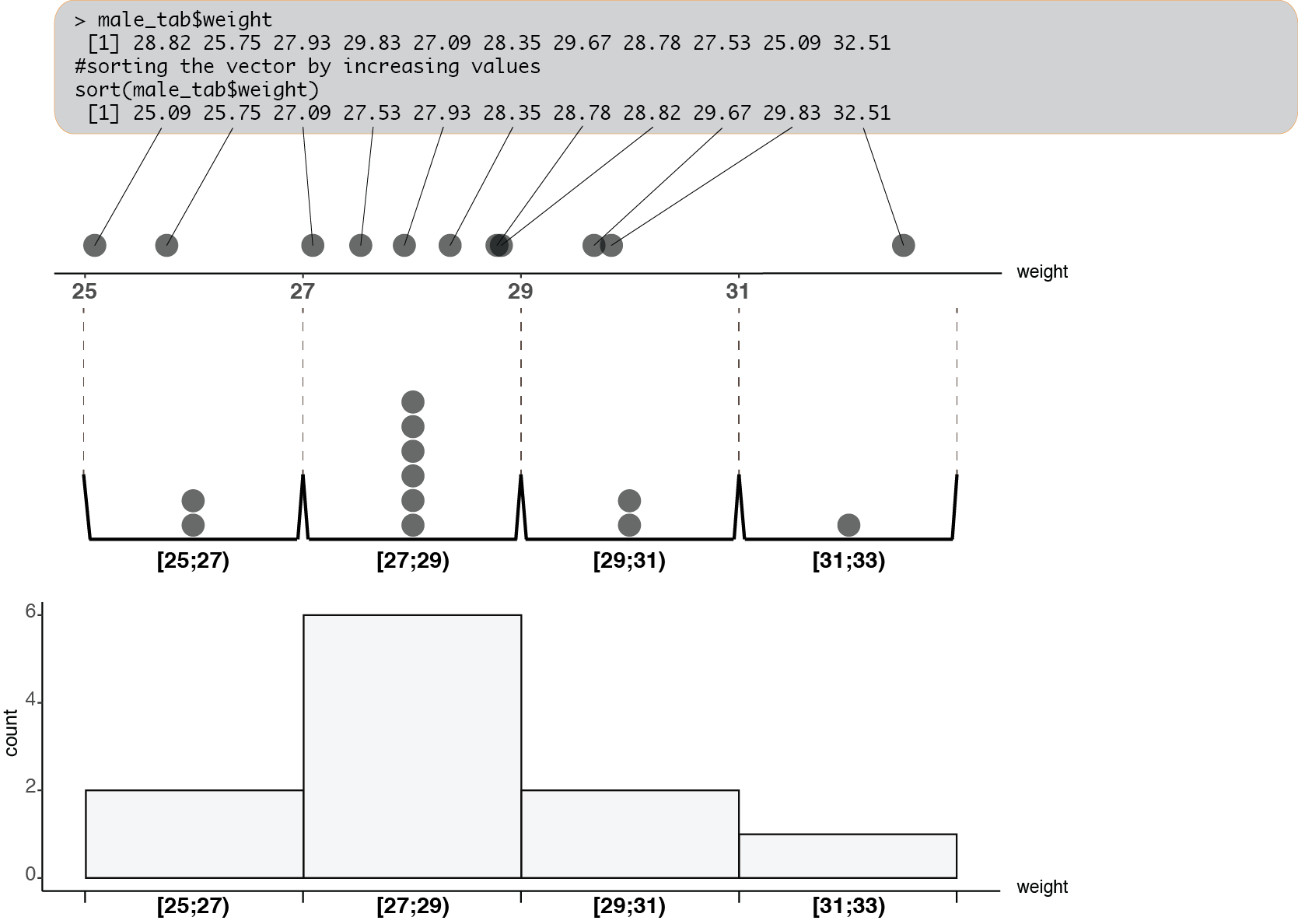
This kind of graphical representation informs us about the distribution of the values in the vector: where values can be found, how broadly they are spread, where they are more concentrated\(\dots\)

Let’s have a quick look at some other measures recorded in our mi data frame.

hist(mi$HeartRate)

hist(mi$Temperature)

The histogram representation reveals striking differences between the distributions of those random variables, and that of the ages.

7.2.1.2 Numerical summaries

A distribution can also be characterized using numbers, such as the mean value, and others. Some of these numbers can be obtained using the summary function, in the form of a named vector:

summary(ages)

   Min. 1st Qu.  Median    Mean 3rd Qu.    Max. 
  20.17   35.83   47.71   46.49   58.35   69.75 

summary(mi$HeartRate)

   Min. 1st Qu.  Median    Mean 3rd Qu.    Max. 
  37.00   54.00   58.00   59.21   65.00  100.00 

summary(mi$Temperature)

   Min. 1st Qu.  Median    Mean 3rd Qu.    Max. 
  35.70   36.20   36.40   36.43   36.60   37.70 

We will soon learn in more details what all these values mean.

We can see that these summary values differ. This reflects differences in the shapes of the histograms and in values on their \(x\)-axes.

The histogram and these summary values are our first step at practicing descriptive statistics.

7.2.2 Describing qualitative data

Now what happens in the case of discrete or qualitative variables?

We can try the summary function on other columns of the data frame:

smoking <- mi$Smoking
summary(smoking)

Active     Ex  Never 
   161    223    432 

sex <- mi$Sex
summary(sex)

Female   Male 
   417    399 

summary gives different kinds of results, depending on the kind of data it received. Here, the data was encoded as factors, a kind of value in R that we haven’t discussed in details yet. Factors are very well suited to represent qualitative variables. This is what is obtained by default for columns containing text in a table loaded in R.

When given factors summary gives the number of individuals falling into each category, or level.

7.2.2.1 Counting using table

We can obtain the same information (in a slightly different form) using the table function:

table(smoking)

smoking
Active     Ex  Never 
   161    223    432 

table(sex)

sex
Female   Male 
   417    399 

Contrary to summary, table works the same with any kind of vector, not just factors. It can be used to count Booleans, strings, numbers\(\dots\) Use it!

Values from a table can be extracted using the corresponding labels, like with named vectors:

counts_smoking <- table(smoking)
counts_active <- counts_smoking["Active"]
counts_active

Active 
   161 

counts_inactive <- counts_smoking[c("Ex", "Never")]
counts_inactive

smoking
   Ex Never 
  223   432 

How would you obtain the total number of inactive smokers ?

Hint

The sum function works on columns of a table of counts:

sum(counts_inactive)

[1] 655

Using table, a contingency table can be created to highlight the interrelation between two variables. In our case, we can create such a contingency table to link the two variables: smoking habits and sex.

table(mi$Sex, mi$Smoking)

        
         Active  Ex Never
  Female     77  95   245
  Male       84 128   187

This table displays the number of individuals observed to have a particular combination of factors. This type of table is used to study the association between two kinds of classification (for instance, classification according to the sex, and classification according to the smoking habits). It is used in particular in Fisher’s exact test.

For the contingency table to make sense, the arguments should be vectors corresponding to measures made over the same series of individuals. In particular, the order of the individuals should be the same in all the vectors.

7.2.2.2 The barplot

To visualize the distribution of categorical data, the barplot function can be used with a table of counts. The result is a graph where each category will be represented by a bar:

barplot(counts_smoking)

barplot(table(sex))

Do not use barplots for non-discrete data! Barplots are not histograms:

• The bars are not contiguous.
• The order of the categories on the \(x\)-axis of a barplot can be changed, not the order of the bins in a histogram.

The first barplot

The first documented barplot is believed to occur in William Playfair’s “The Commercial and Political Atlas” [@Playfair1801].

Playfair’s barplot of imports and exports of Scotland.

7.2.3 From data distribution to population model

One important use of descriptive statistics is to help us choosing the correct tools for later analyses. One aspect is to characterise our samples in terms of the distribution of its values. The distribution of the values in the sample may then suggest ways to model the distribution of the values in the population. This distribution model will be an essential tool in later phases of statistical analysis.

The word “distribution” can be used for two different but related ideas:

• How the values are distributed in a sample (empirical distribution).
• How the values would be distributed if the random variable from which our sample was observed behaved according to certain rules, to a certain model (theoretical distribution).

In the latter sense, a distribution is characterized in terms of probabilities. What is the probability to observe a given value, or to observe a value within a given range?

We will now present some common ways to obtain a distribution to model a random variable.

7.2.4 Discrete distributions

Discrete distributions will be preferred to model naturally discrete quantities (such as numbers of heads on hydras or numbers of popes at certain times in history) that will be represented using integral numbers. They can also be used for some continuous aspects of the physical world that are typically modelled using discrete classes, such as colours (the spectrum of radio-frequencies is continuous, but it is often more practical to score observations according to a discrete set of colours).

A model for a discrete distribution would consist in associating each possible value with the probability of obtaining it when randomly sampling an element from the population.

For instance, the “Milieu Intérieur” data frame contains information regarding individual’s relationships with smoking. This is scored using three categories (a factor with three levels, in R terminology):

• Active, for active smokers;
• Ex, for people that used to smoke but no longer do;
• Never, for people that never got into smoking.

If we wanted a model for this random variable, we could associate each category with a number, between \(0\) and \(1\), and such that the three numbers sum to \(1\) (this is a required property for probabilities). Determining the values for these numbers could be done in various ways (using a priori knowledge, estimating the values from the sample, \(\dots\)).

For instance, we could just use the proportions of each category in the sample as probabilities for our model. This can be computed as follows:

counts_smoking <- table(smoking)
counts_smoking

smoking
Active     Ex  Never 
   161    223    432 

nb_observations <- sum(counts_smoking)
nb_observations

[1] 816

proportions_smoking <- counts_smoking / nb_observations
proportions_smoking

smoking
   Active        Ex     Never 
0.1973039 0.2732843 0.5294118 

Besides using such empirical probabilities to build a model, there are various well studied classical discrete distributions available: Bernoulli, binomial, uniform, Poisson\(\dots\)

Their ability to be mathematically described reflect some “rules”, some regularities or mechanisms, in the process underlying the random variable to which they are associated. This is what makes them useful to extrapolate beyond simple empirical probabilities. Indeed, empirical probabilities will fit the sampled data perfectly, but these probabilities will likely not reflect what happens at the whole population level (especially if the sample is small), resulting in poor behaviour in later phases of statistical analyses. This is sometimes called “over-fitting”.

We will now briefly present a few classical and simple discrete probability distributions.

7.2.4.1 Uniform distribution

This represents the probabilities of equally probable discrete events. Under such a distribution, if there are \(N\) mutually-exclusive events, each one has a probability of \(\frac{1}{N}\). The only parameter needed to use this distribution as a model is \(N\), the number of possible events.

For instance, the outcome of the throw of a standard dice is quite well modelled by a uniform distribution with 6 equally probable events (that we can label using the numbers \(1\) to \(6\)):

7.2.4.2 Bernoulli distribution

This represents the probabilities of a pair of mutually exclusive events. This very simple model has one parameter: the probability of one of the events (that is typically noted \(p\)). The probability of the other event is then \(1 - p\).

For instance, if we are interested in the probability of left-handedness, someone randomly drawn from a population could be either left-handed (\(L\)) or not (\(\bar{L}\)).

The following would be the distribution of probabilities if the probability of left-handedness was \(\frac{1}{10}\):

If we wanted a model for the Sex column of our mi data frame using a Bernoulli distribution, we could use the proportion of females as parameter p. Compute this proportion using the sex vector.

Hint

sex_counts <- table(sex)
nb_females <- sex_counts["Female"]
prop_females <- nb_females / sum(sex_counts)
prop_females

   Female 
0.5110294 

7.2.4.3 Binomial distribution

This represents the probabilities of achieving a certain number of times a given outcome in a series of drawings from the same Bernoulli distribution. This model takes two parameters: the number of drawings, and the probability of the outcome of interest in the underlying Bernoulli distribution.

For instance, assuming a coin flip can either result in a head or a tail, with equal probability (and nothing else), the probability of obtaining a head would be \(\frac{1}{2}\). (This is a case of discrete uniform and Bernoulli distribution at the same time.)

The probabilities of obtaining a certain number of tails in 5 coin flips can therefore be modeled using a binomial distribution with 5 events:

7.2.5 Continuous distributions

Physical measures such as sizes, weights, or durations are continuous by nature. Assuming an arbitrarily high precision, they could take any value between a pair of (possibly infinite) real numbers.

For such measures, each value is one possibility among an infinity of others. It is therefore not useful to associate individual probabilities to each possible value because the probability of one value among an infinity of other possibilities is infinitesimal.

A model for a continuous random variable should instead associate probability densities to real numbers in the (possibly unbound) range of possible values for that variable, in the form of a probability density function.

Let’s take again our male mice weights example and try to figure out what a probability density is.

As we have seen with the smoking habits example, a probability can be estimated from empirical data by taking the proportions of observations within each category. The same can be done with continuous data, using histogram bins instead of categories.

Now, a probability “density” can be derived from these per-bin probability estimates, by scaling them by the bin widths.

download figure

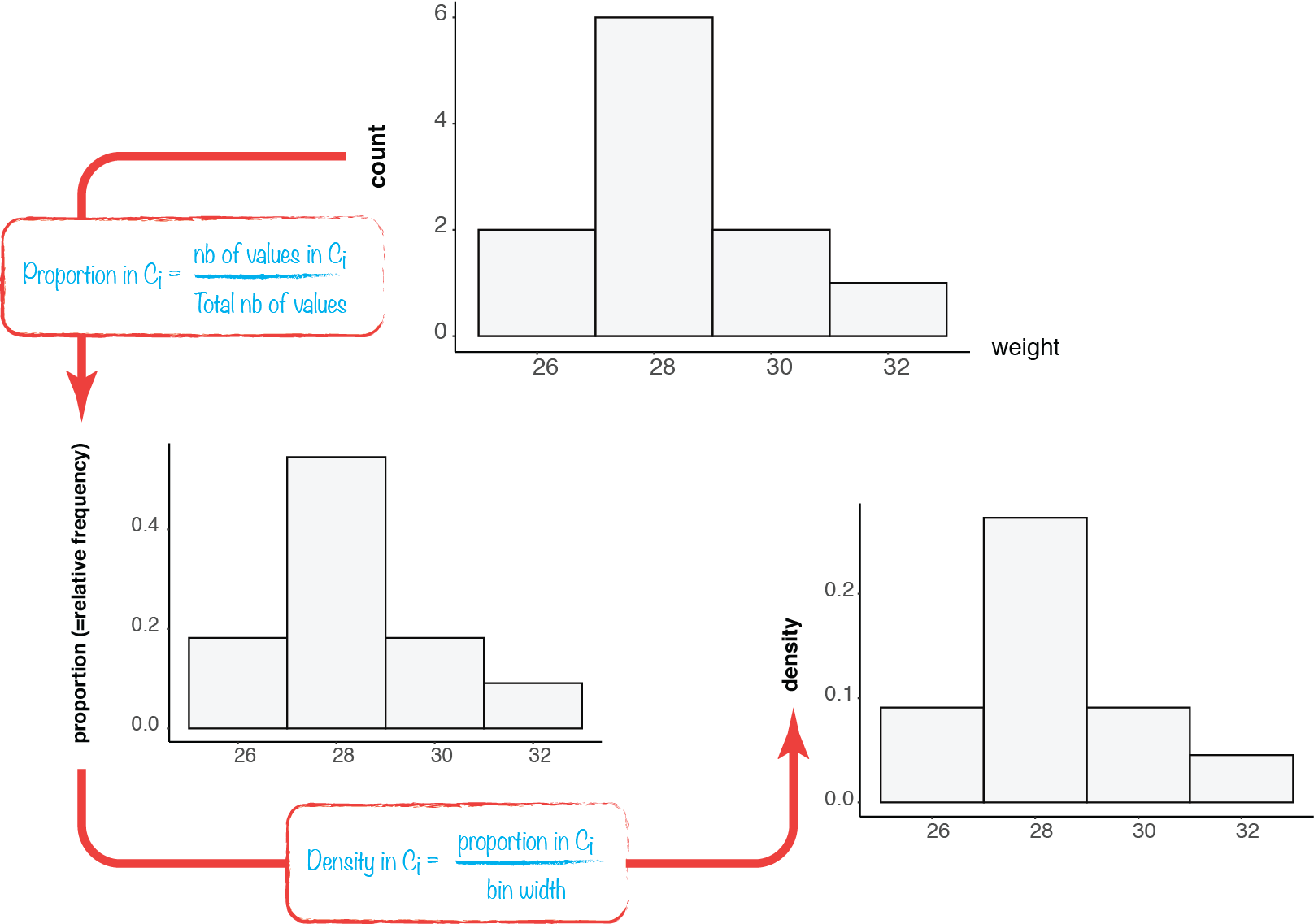
Here, we transform the probabilities of certain ranges of weights into a kind of probability “per unit of weight”.

Numerical analyses techniques exist that can smooth these densities to extrapolate a distribution for the underlying population. This is a way to provide an empirical model of continuous distribution for the population.

In R, the density function can make such an estimation of densities, which can be plotted using the plot function:

plot(density(male_tab$weight))

(The plot function is a versatile function that tries to guess what kind of graph we want based on the nature and numbers of arguments.)

download figure

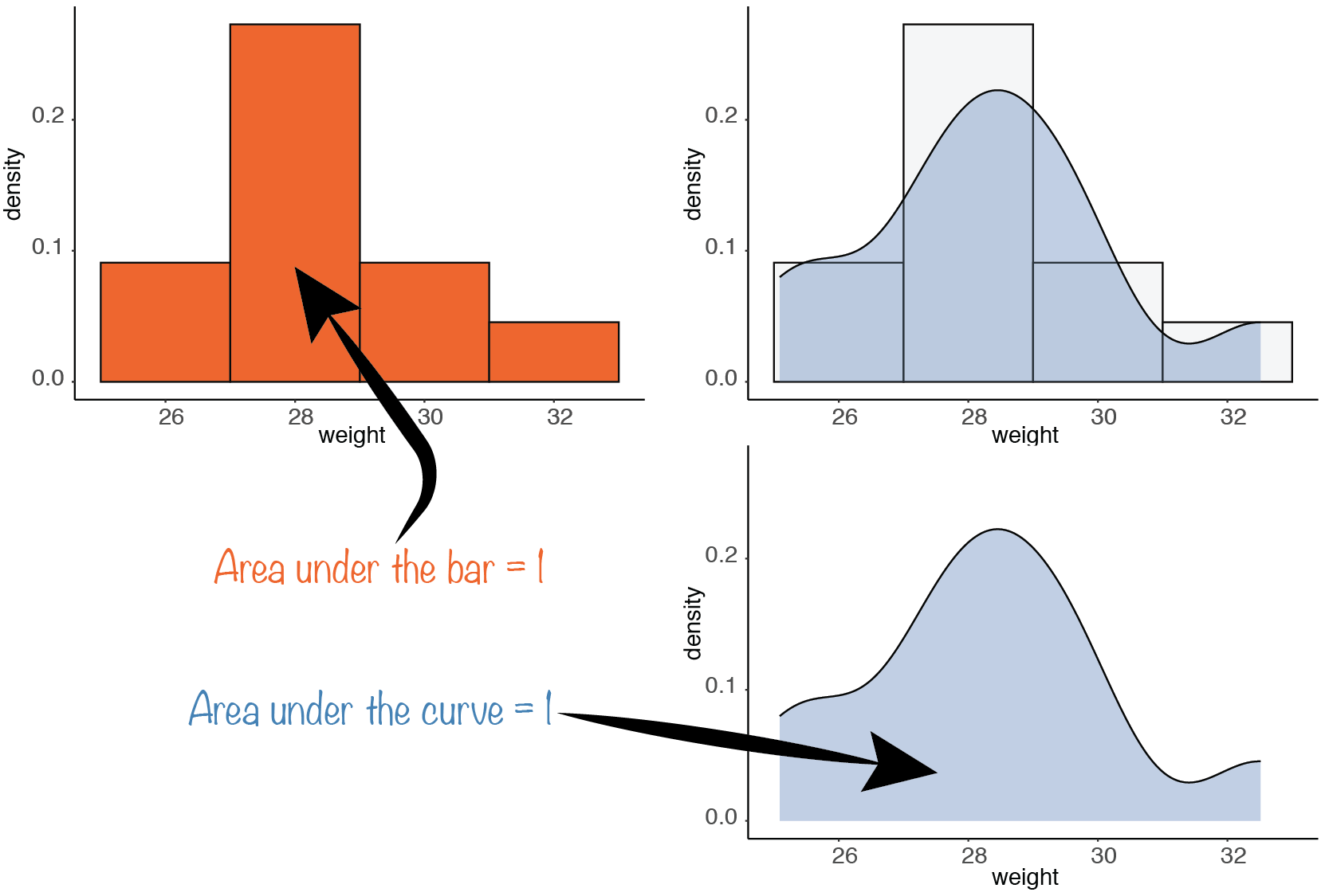
An important property is verified for both the smooth and non-smooth densities: The total area under the curve (sum of the areas of the bars, in the non-smooth case) is \(1\).

In mathematical terms, a probability density function is a positively-valued function that, once integrated between two values of its domain of definition, will give the probability to sample a value between these two boundaries. Therefore, the area below the whole curve corresponds to the probability that a sampled value will be “somewhere where values are possible”, which is \(1\).

Mathematical integration of a function can be visualized on the function’s graph as the area under the curve between the boundaries:

As we can see, on the above example, for a same interval width (\(2\)), the probability of a value between \(-4\) and \(-2\) is much lower than the probability of having a value between \(0\) and \(2\). This reflects the fact that the above probability density is higher around zero than far from it.

Why the area under the curve?

For a function with positive values (for instance, a probability density) an integral can be seen as the sum of the surfaces of (infinitely many) infinitesimally narrow rectangles whose heights are given by the function.

\[P(a \le x \le b) = \int_{a}^{b}f(x)\:dx = \lim_{w\rightarrow0} \sum_{i=0}^{\frac{b-a}{w} - 1}(f(a+i\times w)\times w)\]

This intuitively explains why the probability of drawing a value between two boundaries can be visualized as the area under the curve between those boundaries.

As was the case for discrete distributions, some classical continuous distributions exist. For instance: Continuous uniform, Gaussian (or Normal), Chi-squared, Student, Fisher\(\dots\)

They may prove helpful when trying to generalize beyond experimentally derived probability densities.

We will now briefly present a few of them.

7.2.5.1 Continuous uniform distribution

This distribution is characterized by an equal probability density all along a given interval. It is characterized by a \(min\) and a \(max\) parameters, delimiting that interval.

Here is the curve of the density function for the continuous uniform distribution on the \([-1; 1]\) interval:

The density is easy to express in terms of the \(min\) and the \(max\) parameter: \(\frac{1}{max - min}\).

Check that this is the case on the above figure, and compute the area of the rectangle delimited by the density curve and the \(x\)-axis.

Hint

Here, \(min\) is \(-1\) and \(max\) is \(1\). So \(max - min\) is \(2\), hence the density of \(1/2 = 0.5\).

The area of the rectangle is \(2 \times 0.5\), that is \(1\).

7.2.5.2 Normal distribution

This is arguably the most famous family of continuous probability density functions. It is also known as “Gaussian” (from Gauss, a scientist who discovered it trying to characterize the distribution of measurement errors). It is sometimes also qualified as “Bell shaped”, for the shape of the curve of its probability density function:

This distribution is symmetrical takes two parameters, the mean (determining around what value it is centered) and the standard deviation (determining how spread it is around the mean). We will discuss those terms with more details later.

The above curve is the one for the standard normal distribution, that is, the one whose mean is \(0\) and standard deviation is \(1\).

Here is what the curves look like with mean \(0\) and standard deviations \(0.5\), \(1\) and \(2\):

If a random variable is modelled using a normal distribution, it is often useful to transform the data so that the standard normal distribution can be used.

This standardization can be done by simply subtracting the mean of the values, so that the values are centered around zero, and then dividing by the standard deviation of the values (more about this soon), so that the standard deviation now becomes \(1\). This can be called a scaled variable. (For French speakers, this is called “centrer et réduire”, and the result is a “variable centrée réduite”.)

This kind of transformation can be applied even if the variable does not follow a normal distribution. Just keep in mind that the result will not follow a standard normal distribution, in that case.

7.2.5.3 Student’s t-distribution

This distribution was discovered by William Sealy Gosset, an employee of the Guinness brewery who published his work under the pseudonym “Student”.

Like the standard normal distribution, it is bell shaped and centered around zero. However, it is more widely spread.

It takes a parameter called “degree of freedom”, which is an integral number. The higher the degree of freedom, the lower the dispersion of the values, and the closest to the standard normal distribution.

Here is a Gaussian distribution, together with t-distributions of various degrees of freedom:

7.2.5.4 Chi-squared distribution

The Chi-squared distribution (or \(\chi^2\)-distribution) also has a parameter named “degree of freedom”. If \(df\) is the degree of freedom, the particular distribution can be noted \(\chi_{df}^2\), and is the distribution of the sum of \(df\) squared independent random variables following the standard normal distribution.

For instance, if a variable is modelled using a normal distribution, centering the values (by subtracting the mean), then normalizing (by dividing by the standard deviation), and finally squaring, would result in a random variable that is expected to follow a \(\chi_{1}^2\) distribution. This has various applications.

As a sum of squares, this probability density is only defined for positive numbers. Here are the curves for various degrees of freedom:

7.2.6 Vectors of random values

It can sometimes be useful to generate data following certain probability distributions.

R provides a family of functions whose name starts with “r”, and then something reminding the name of a theoretical distribution: rbinom for the binomial distribution, rnorm for the normal distribution, rt for Student’s t-distribution, rchisq for the Chi-squared distribution\(\dots\)

These functions generate vectors of random values drawn from the corresponding distribution.

For instance, the rnorm function generates a vector of random values from a standard normal distribution (mean 0 and standard deviation 1):

ten_norm <- rnorm(10)
ten_norm

 [1] -0.4764353  1.5712980 -0.5405243 -0.5895441  1.0954162 -0.6731219
 [7]  0.1096119  1.0659272  0.1661113  0.2101096

The argument is the number of values to draw from the distribution.

We can quickly visualize the distribution of the obtained numbers using the hist function:

hist(ten_norm)

We can change the parameters of the normal distribution using the mean and sd optional arguments. mean and sd have default values of 0 and 1 respectively, so that rnorm draws from the standard normal distribution by default.

For instance, we can generate values from a normal distribution of mean \(10\) and standard deviation \(0.1\) as follows:

ten_norm_2 <- rnorm(10, mean = -4, sd = 0.1)
ten_norm_2

 [1] -3.934045 -4.089639 -4.163901 -3.755335 -3.892571 -3.983323 -3.940167
 [8] -4.180485 -4.114692 -3.950806

The histogram should reflect the change in parameters:

hist(ten_norm_2)

Use the help of the rbinom function (?rbinom) to find how to generate 32 random values drawn from a binomial distribution modeling the number of tails obtain when flipping five coins. Create a flip_5_32 vector and make a barplot to represent the obtained distribution.

Hint

flip_5_32 <- rbinom(32, size = 5, prob = 0.5)
barplot(table(flip_5_32))

7.3 Location

One of the aspects by which a distribution of values can be characterized is its “central tendency”, or “location”. This is a way to estimate what a “typical” value from that distribution would be. There are several approaches to do this kind of estimation. The most commonly used location parameters are the mean and the median.

7.3.1 Arithmetic mean

The best known location descriptor is the (arithmetic) mean (or “average”) of the values. For a sample of values, it can be computed as the sum of the values, divided by the number of values.

The mean \(m\) of a sample with \(n\) values (noted \(x_1\), \(\dots\), \(x_n\)) can be expressed as follows:

\[m = \frac{x_1 + ... + x_n}{n}\] or (using the mathematical notation for a sum): \[m = \frac{\sum_{i=1}^{n}x_i}{n}\]

Mean of a theoretical distribution

The mean (\(\mu\)) of a theoretical distribution can be computed from its probability (\(P\)) or probability density (\(f\)) function (for discrete or continuous distributions, respectively).

Given a discrete probability distribution (represented by a probability function \(P\) associating a probability to each individual possible value), the mean (\(\mu\)) of a population can be expressed as a weighted sum of values:

\[\mu = \sum_{x \in \Omega} x\:P(x)\] where \(\Omega\) represents the set of all possible values.

Similarly, in the case of a continuous probability distribution (represented by a probability density function \(f\)), the mean of the population can be expressed using a weighted integral over the domain of definition:

\[\mu = \int_{x=a}^{b}x\:f(x)\:dx\] where \(a\) and \(b\) are the (possibly infinite) lower and upper boundaries of the range of possible values.

However, in practice, the above \(P\) or \(f\) functions will actually be specified in terms of parameters such as their mean or standard deviation.

These parameters will have to be estimated from the sampled data.

When using a theoretical distribution to model a population, the theoretical distribution has to be tuned using parameters. These parameters are often noted using Greek letters.

For instance, to have the theoretical distribution centered around the same values as the data, one would typically use the mean as a tuning parameter. The (unknown) mean of the population would be the ideal value for the mean parameter (noted using the Greek letter \(\mu\)). It will be estimated using the (known) sample mean (\(m\)). Such an estimated mean is sometimes noted \(\hat{\mu}\), to distinguish it from the real population mean \(\mu\). \(\hat{\mu} = m\). If the sample is not biased, \(\hat{\mu}\) for large samples will tend to be close to \(\mu\).

Estimators obtained from a sample are often noted with decorations such as \(\hat{\phantom{\mu}}\) to distinguish them from the parameters of mathematical models chosen to represent probability distributions of the population.

About Greek letters

You may have noticed that mathematical traditions heavily rely on the use of Greek letters:

• The first two letters “alpha” (\(\alpha\)) and “beta” (\(\beta\)) are often used for parameters.
• Capital “gamma” (\(\Gamma\)) is sometimes used to denote a particular distribution.
• “Deltas” (\(\Delta\) and \(\delta\)) are used for large and small differences respectively.
• “Epsilon” (\(\varepsilon\)) is used for very small values.
• “Theta” (\(\theta\)) can be used for an angle but is also widely used for other parameters.
• “Lambda” (\(\lambda\)) is used to parametrize the Poisson distribution, as well as in theoretical computer sciences.
• Greek letter “mu” (\(\mu\)) is typically used to represent a mean, hence \(\hat{\mu}\) for the estimation of a mean.
• You already know “pi” (\(\pi\)) whose capital counterpart \(\Pi\) is often used to denote a product.
• “Rho” (\(\rho\)) is used for correlation coefficients.
• We have recently met with capital “sigma” (\(\Sigma\)), standing for a sum, and we will later encounter it’s smaller counterpart \(\sigma\), which stands for standard deviation.
• “Tau” (\(\tau\)) usually stands for a time parameter.
• “Chi” (\(\chi\)) is usually squared to denote the theoretical distribution of sums of squared normal distributions.
• “Phi” (\(\varphi\)) is sometimes used for angles\(\dots\)
• as well as “omega” (\(\omega\)), which, last but not least, is also used for whole universes of possibilities in its capital form (\(\Omega\)).

Can you compute the mean of the values in the ages vector?

Hint

We have already seen the length function, that can be used to get the number of elements in a vector, and the sum function, that sums its elements.

To compute the mean of the values in a vector, we can simply apply the definition of the mean, using sum and length:

sum(ages) / length(ages)

[1] 46.48571

We do not need to manually compute the mean using sum and length. There is actually a mean function for that:

mean(ages)

[1] 46.48571

We can try to apply mean on a vector of Booleans:

mean(ages > 30)

[1] 0.8504902

What does this value represent?

Hint

This is the proportion of individuals above the age of 30 (number of TRUE divided by number of elements).

Can you find the mean of the ages, excluding young people (assuming old age starts at 64)?

Hint

mean(ages[ages >= 64])

[1] 66.32543

Other types of means

You may occasionally encounter other types of means than the arithmetic mean, in particular when dealing with certain kinds of positive values.

While the arithmetic mean summarizes data based on their sum, the geometric mean summarizes data on the basis of their product. The product of the values in a vector can be obtained using the prod function. To obtain something in the same unit as the summarized values, the \(n^{th}\) root of it is taken, where \(n\) is the number of elements. This is equivalent to computing the \((1/n)^{th}\) power of the product (using the ^ exponentiation operator):

prod(ages) ^ (1 / length(ages))

[1] Inf

However, due to limitations in the way numbers are represented in a computer, R might consider that a large value (such as the product of the ages of many adults) amounts to infinity (Inf).

To circumvent this issue, it is possible to work with a log-transformation of the numbers.

In the log-transformed space, a product becomes a sum. We can verify this on a small vector of ages, using the log function:

ages_toy <- c(34, 4, 18, 5, 56, 41, 23, 101)
log(prod(ages_toy))

[1] 24.902

sum(log(ages_toy))

[1] 24.902

Still in the log-transformed space, an exponentiation becomes a product:

log(prod(ages_toy) ^ (1 / length(ages_toy)))

[1] 3.11275

sum(log(ages_toy)) * (1 / length(ages_toy))

[1] 3.11275

We recognize here the formula of the arithmetic mean. So the log-transformed version of the geometric mean is the arithmetic mean of the log-transformed values:

log(prod(ages_toy) ^ (1 / length(ages_toy)))

[1] 3.11275

mean(log(ages_toy))

[1] 3.11275

Transforming the result with exp (the inverse function of the log), gives back the geometric mean:

prod(ages_toy) ^ (1 / length(ages_toy))

[1] 22.4828

exp(mean(log(ages_toy)))

[1] 22.4828

We can now try this with the large vector of ages:

exp(mean(log(ages)))

[1] 44.1649

The harmonic mean is the inverse of the arithmetic mean of the inverses of the values:

1 / mean(1 / ages)

[1] 41.62352

(1 / ages is a vector containing the inverses of each of the values in ages.)

7.3.2 Median

Another descriptor for the location of a distribution is the median, that is, the value that separates the distribution in two halves of equal numbers of elements.

Two cases may be distinguished:

• If there are an odd number of values, the median is the middle value.
• If there are an even number of values, one usually takes the average of the two middle values.

Determine the median of our small ages_toy vector.

Reminder:

ages_toy <- c(34, 4, 18, 5, 56, 41, 23, 101)

Hint

length(ages_toy)

[1] 8

We have 8 values.

Let’s sort them:

sort(ages_toy)

[1]   4   5  18  23  34  41  56 101

Since the number of values is even, the median is somewhere between the two middle values 23 and 34.

We can take the mean of these two numbers:

half_len <- length(ages_toy) / 2
mean(sort(ages_toy)[c(half_len, half_len + 1)])

[1] 28.5

Automating the computation of the median

In R, it is possible to create custom functions. Just to give you a taste of what it looks like, here is how we could create a function that automates the computation of the median of a vector:

my_median <- function(v) {
    #                 ^
    #                 |
    # The argument given when calling the function
    # will be stored in the "local" variable v during
    # the computation of the function's result.
    # We can compute the length of the given vector.
    #          |
    #          v
    l = length(v)
    # The last executed computation will determine
    # the result of the function call.
    # The
    # if (<some Boolean>) {<some computation>}
    # else {<some other computation>}
    # construct allows us to have two alternate computations
    # for the result of the function.
    # l %% 2 gives the remainder of the integer division of l by 2.
    # If that remainder is zero, it means that l is even.
    if (l %% 2 == 0) {
        # l is even.
        # We compute the mean of the 2 middle values:
        mean(sort(v)[c(l / 2, l / 2 + 1)])
    }
    else {
        # l is odd.
        # We just extract the middle value:
        sort(v)[(l + 1) / 2]
    }
}
# Now let's test it:
my_median(1:4)

[1] 2.5

my_median(1:5)

[1] 3

# It works! Cool, isn't it?

Contrary to the arithmetic mean, the median cannot be computed using a simple mathematical formula. It is a bit painstaking to compute a median “manually”. Fortunately, R provides the median function, that does all the tedious work of searching this value for us:

median(ages)

[1] 47.71

An important property of the median is that it is less sensitive than the mean to the presence of atypical values (“outliers”).

To illustrate this, let’s consider again our small vector of ages:

ages_toy

[1]  34   4  18   5  56  41  23 101

Suppose that our data was obtained from a table where a reporting error occurred, so that we instead obtained this vector:

ages_wrong <- c(34, 4, 18, 5, 560, 41, 23, 101)

If a value above the median is erroneously increased, or a value below the median is erroneously decreased, the median will not be affected.

The mean, however, will change:

median(ages_toy)

[1] 28.5

median(ages_wrong)

[1] 28.5

mean(ages_toy)

[1] 35.25

mean(ages_wrong)

[1] 98.25

Here is another small example, this time with an odd number of elements. The median is indeed one of the elements:

powers <- c(1, 2, 4, 16, 256)
median(powers)

[1] 4

Notice how “skewed” the above distribution is. The median is much closer to the minimum than to the maximum value. What about the mean?

mean(powers)

[1] 55.8

The above example shows that a location estimator is far from enough to characterize a distribution, and may sometimes not be very useful.

7.3.3 Mode

The mode of a distribution of value is the most frequent value, the most likely to be sampled.

Considering the mode as a location parameter most makes sense for densely sampled discrete distribution. For small samples of values taken from a large or a continuous range, no meaningful mode is likely to emerge, as most sampled values will be unique. However, if the global population from which such a sample is obtained is modeled using a continuous distribution, the theoretical mode can be meaningful and will be the value at which the corresponding probability density is highest.

There is no R function to compute the mode (at least by default). We will soon see how to compute the mode of a sample of values.

7.4 Dispersion

The location of a distribution of values is important to estimate, but distributions with the same location can actually be very different. For instance, the values can be all close to the location parameter, or on the contrary vastly dispersed. This will have an important influence on the outcome of statistical tests.

7.4.1 Range

One very simple way to describe the dispersion of the data is to extract its extreme values:

min(ages)

[1] 20.17

max(ages)

[1] 69.75

range(ages)  # min and max in one function

[1] 20.17 69.75

The range function in R gives the extreme values from a distribution, whereas in statistics, the term “range” is used to refer to the breadth of the distribution, that is, the difference between the highest and the lowest value:

range_ages <- max(ages) - min(ages)
range_ages

[1] 49.58

It is also possible to use the diff shortcut function:

diff(range(ages))

[1] 49.58

Can you compute the index (or indices) of the lowest value (or values) in the age vector?

Hint

which(ages == min(ages))

[1] 21

There are shortcut functions for this common type of operation:

which.min(ages)

[1] 21

which.max(ages)

[1] 688

min, max and range are obviously very sensitive to the presence of outliers.

Find the mode of the smoking vector.

Hint

This can be done with the new tools we just learned about:

which.max(table(smoking))

Never 
    3 

# Or, using the computed empirical probabilities:
which.max(proportions_smoking)

Never 
    3 

Here, we obtain a named vector with one element. The name is above, the index of the highest element onf the table below. To extract the name, we can use the names function. Both can be used to extract the actual counts from the table:

table(smoking)[which.max(table(smoking))]

Never 
  432 

table(smoking)[names(which.max(table(smoking)))]

Never 
  432 

7.4.2 Variance and standard deviation

The variance is a measure of dispersion with respect to the mean. It represents a “typical” value for the (squared) distances to the mean.

The variance \(s^2\) of a sample (of size \(n\)) can be computed as the arithmetic mean of the squared deviations of its values (noted \(x_1\), \(\dots\), \(x_n\)) from its mean \(m\).

\[s^2 = \frac{(x_1 - m)^2 + \dots{} + (x_n - m)^2}{n}\] or: \[s^2 = \frac{\sum_{i=1}^{n}(x_i - m)^2}{n}\]

Some theoretical distributions will have a variance (\(\sigma^2\)) tuning parameter, to make the values more or less spread around the mean.

If we had access to the full population, its variance would be the perfect value for this parameter. However, we only have access to the variance of a sample.

Unfortunately, unless the sample mean happens to be exactly the real (and unknown) population mean, the sample variance will be an under-estimation of the population variance. This comes from the fact that the mean of a sample is the value that minimizes the sum of squared distances to the sampled values.

To estimate the population variance, a slightly modified formula should be used:

\[\hat{\sigma^2} = \frac{(x_1 - m)^2 + \dots{} + (x_n - m)^2}{n - 1}\] or: \[\hat{\sigma^2} = \frac{\sum_{i=1}^{n}(x_i - m)^2}{n - 1}\]

This is the formula implemented in the var function in R:

sum((ages - mean(ages)) ^ 2) / (length(ages) - 1)

[1] 191.9444

var(ages)

[1] 191.9444

The two formulas will give close values for large sample sizes, reflecting the fact that population mean estimations will tend to be more accurate using large samples.

You should use the second one when you need a variance parameter to tune a theoretical distribution. That is why this is the formula implemented in var.

The standard deviation can be computed by taking the square root (sqrt function in R) of the variance. This provides a dispersion estimation in the same unit as the studied values, and can be directly obtained using the sd function.

sqrt(var(ages))

[1] 13.8544

sd(ages)

[1] 13.8544

Greek letter \(\sigma\) (“sigma”) stands for “standard deviation” in the notation for the variance (\(\sigma^2\)).

Now that you know how to compute a mean and a standard deviation, create a vector representing a standardization of the weights of the male mice.

Hint

As we have seen previously, one should first compute the mean and standard deviation of the values.

mean_weight <- mean(male_tab$weight)
sd_weight <- sd(male_tab$weight)

Then, we can center the values around their mean, and scale to the standard deviation:

standardized_weights <- (male_tab$weight - mean_weight) / sd_weight

We can check that the mean of the resulting values is indeed zero (or something very close, depending on the precision of real number representation in the computer), and its standard deviation is \(1\):

mean(standardized_weights)

[1] -2.304422e-17

sd(standardized_weights)

[1] 1

7.5 Quantiles

For a given distribution, any probability can be associated to a quantile. The quantile at probability \(p\) (or quantile of order \(p\)) is the value \(Q\) such that a proportion \(p\) of the values in the distribution of interest are below or equal to \(Q\). Hence, there is a proportion \(1 - p\) of the values in the distribution that are equal or above of \(Q\).

We have already seen an example of quantile: The median of a distribution is its quantile at probability \(0.5\).

Indeed, the median divides a distribution in two halves with equal number of points. The proportion of the values that are below the median is \(0.5\), and the proportion of the values that are above is \(1 - 0.5\).

Some other widely used quantiles are the first quartile (at probability \(0.25\)) and the third quartile (at probability \(0.75\)). Together with the median (which is the second quartile), they cut the distribution into four bins of equal number of counts.

If we have a density for our population (for instance estimated using the density function), we can have an estimation for the value of any quantile. This can be graphically represented on the plot of the density, as follows:

download figure

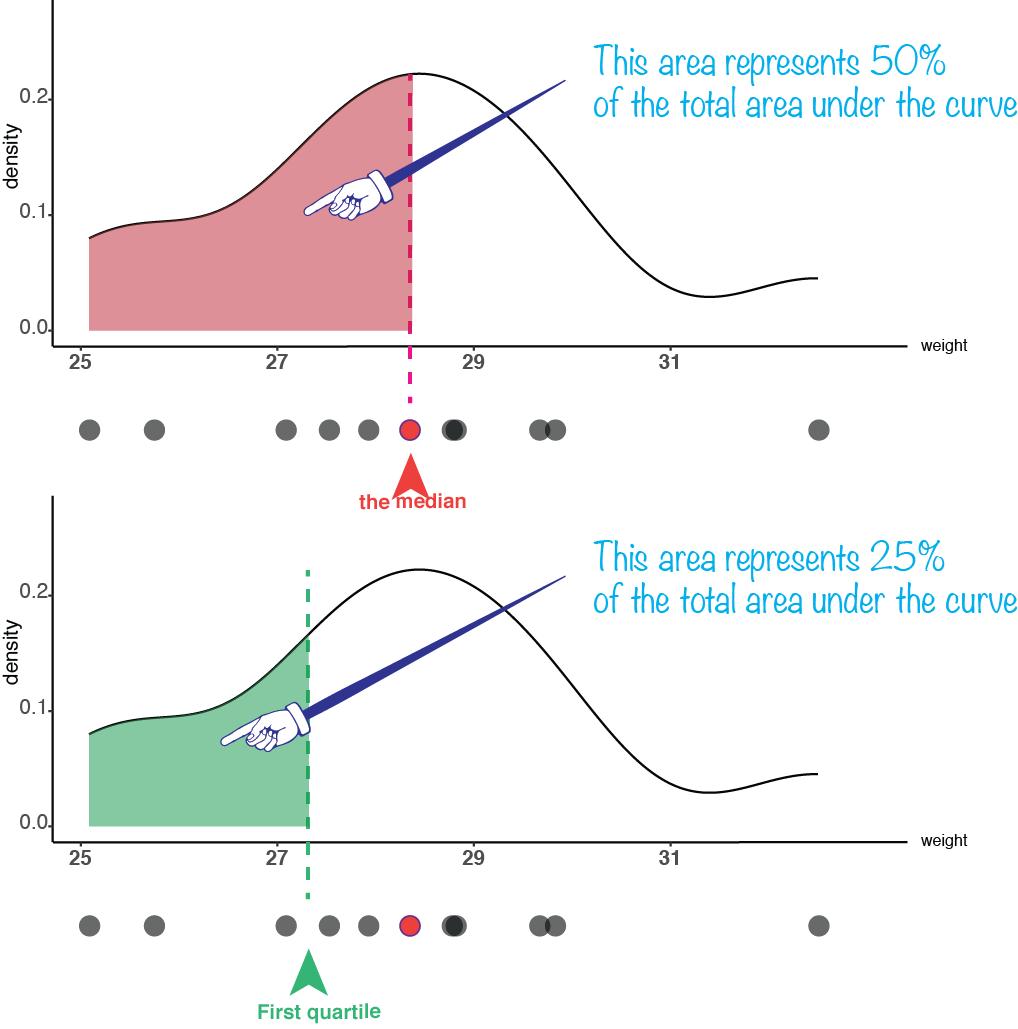
The quantile at a given probability can be estimated using the quantile function:

quantile(male_tab$weight, probs = 0.25)

  25% 
27.31 

quantile(male_tab$weight, probs = 0.5)

  50% 
28.35 

The probs argument specifies the probability whose quantile is desired. It can actually take a vector of probabilities:

quantile(male_tab$weight, probs = c(0.25, 0.5))

  25%   50% 
27.31 28.35 

The result is a vector containing the cut values, with names displayed above those values. The names correspond to the proportion of the values that are below the corresponding quantile.

When a quantile does not correspond to an actual value in the data, several methods exist to choose a value between the two closest data points (taking the average is the simplest one). This may result in differences between tools. For instance, the boxplot function, that we will present soon, uses a different method than the quantile function.

The distribution of values in a sample can be summarized by determining what values cut the distribution into bins of equal size (in terms of numbers of sampled values falling in the bins). These cutting values are quantiles of the distribution corresponding to regularly spaced probabilities.

The cutting of a distribution into quantiles can be more or less fine-grained, depending on the number of bins into which the distribution of values is cut: quartiles, deciles, centiles.

7.5.1 Quartiles

A typical usage is to cut the distribution into four bins and the corresponding quantiles are then called quartiles.

This is what the quantile function reports when the probs argument is not set:

quantile(ages)

     0%     25%     50%     75%    100% 
20.1700 35.8300 47.7100 58.3525 69.7500 

In the above example:

• 0% of the values are below 20.17
• 25% of the values are below 35.83
• 50% of the values are below 47.71
• 75% of the values are below 58.3525
• 100% of the values are below 69.75

This named vector can be handled just like a normal vector (the extracted values will keep the associated names, though):

age_quartiles <- quantile(ages)
age_quartiles["50%"]

  50% 
47.71 

As mentioned before, the 50% quantile actually corresponds to the median (it divides the distribution in two halves).

The 0% and 100% quantiles should correspond to the min and max.

Extract a subset of age_quartiles containing only these two extreme values.

Hint

age_quartiles[c("0%", "100%")]

   0%  100% 
20.17 69.75 

As mentioned earlier, the behaviour of the summary function depends on the type of data on which it is applied. In the case of a vector of numbers, it computes the quartiles (with fancier names than when quantile is used) as well as the mean:

summary(ages)

   Min. 1st Qu.  Median    Mean 3rd Qu.    Max. 
  20.17   35.83   47.71   46.49   58.35   69.75 

7.5.2 Interquartile range (and outlier detection)

Since the min and the max are highly sensitive to the presence of outliers, the only quartiles actually considered in practice are those delimiting 25%, 50% and 75% of the distribution. They are sometimes noted \(\textrm{Q}_1\), \(\textrm{Q}_2\) and \(\textrm{Q}_3\), and the difference between \(\textrm{Q}_3\) and \(\textrm{Q}_1\) is used as a dispersion measure named interquartile range (\(\textrm{IQR}\)): \(\textrm{IQR} = \textrm{Q}_3 - \textrm{Q}_1\)

download figure

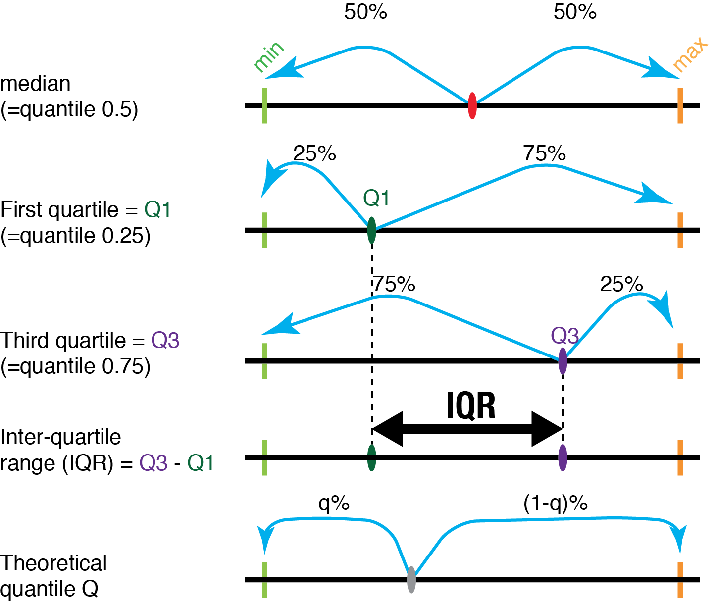
Compute the interquartile range of our ages vector (and put this in a variable named iqr_ages).

Hint

iqr_ages <- age_quartiles["75%"] - age_quartiles["25%"]
iqr_ages

    75% 
22.5225 

Another option can be to use directly the output of the summary function:

iqr_ages <- summary(ages)["3rd Qu."] - summary(ages)["1st Qu."]
iqr_ages

3rd Qu. 
22.5225 

R is trying to help us and decided to keep the name of the first element in our subtraction. Since this actually doesn’t make sense, let’s get rid of it by setting iqr’s name to NULL:

names(iqr_ages) <- NULL
iqr_ages

[1] 22.5225

Guess what? There’s actually an R function to easily get the interquartile range of a vector:

IQR(ages)

[1] 22.5225

Like the standard deviation, the interquartile range is in the same unit as the values. It is less sensitive to the presence of outliers, and is actually used to define a criterion to detect outliers. Typically, values below \(\textrm{Q}_1 - 1.5 \times \textrm{IQR}\) or above \(\textrm{Q}_3 + 1.5 \times \textrm{IQR}\) are considered outliers.

Using this criterion, filter out outliers from our ages_wrong small vector example, into an ages_better vector.

Reminder:

ages_wrong <- c(34, 4, 18, 5, 560, 41, 23, 101)

Hint

First, let’s compute the quartiles of interest and the interquartile range:

Q1 <- quantile(ages_wrong)["25%"]
Q3 <- quantile(ages_wrong)["75%"]
iqr_ages_wrong <- IQR(ages_wrong)

Now we can compute the lower and upper bound of the values we want to keep:

lower_ok <- Q1 - 1.5 * iqr_ages_wrong
upper_ok <- Q3 + 1.5 * iqr_ages_wrong

From this, we can make a Boolean vector indicating where in our ages_wrong vector the values are acceptable:

age_not_outlier <- (lower_ok <= ages_wrong) & (ages_wrong <= upper_ok)

Finally, we can use Boolean sub-setting to create our filtered out vector:

ages_better <- ages_wrong[age_not_outlier]
ages_better

[1]  34   4  18   5  41  23 101

Note that the interquartile range will vary depending on the method used to determine quantiles. Outlier detection will therefore also vary.

7.5.3 Boxplots

The median, quartiles and outliers are represented on graphs called boxplots.

Here is a nice boxplot for our mice weights data, with detailed annotations:

download figure

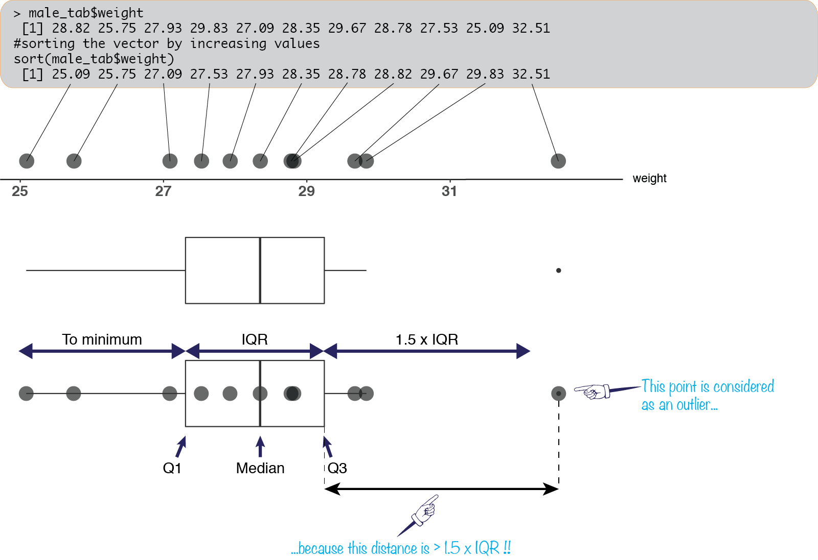
We can make our own boxplots using the boxplot function.

Let’s use it, together with another function, abline, that can add straight lines to a graph:

quartiles_toy <- quantile(ages_toy)
Q0_toy <- quartiles_toy["0%"]
Q1_toy <- quartiles_toy["25%"]
Q2_toy <- quartiles_toy["50%"]
Q3_toy <- quartiles_toy["75%"]
Q4_toy <- quartiles_toy["100%"]
iqr_toy <- IQR(ages_toy)
lower_ok_toy <- Q1_toy - 1.5 * iqr_toy
upper_ok_toy <- Q3_toy + 1.5 * iqr_toy
boxplot(ages_toy,
        ylim = c(
            min(lower_ok_toy, Q0_toy),
            max(upper_ok_toy, Q4_toy)))
abline(
  h = Q0_toy,
  col = "grey", lty = "dashed")
abline(
  h = lower_ok_toy,
  col = "grey")
abline(
  h = Q1_toy,
  col = "green")
abline(
  h = Q2_toy,
  col = "red", lty = "dashed")
abline(
  h = Q3_toy,
  col = "blue")
abline(
  h = upper_ok_toy,
  col = "grey")
abline(
  h = Q4_toy,
  col = "grey", lty = "dashed")

The h argument of abline is used to indicate the \(y\)-axis coordinate of a horizontal line to draw. There is also a v argument, to specify the \(x\)-axis coordinate of a vertical line. Many plotting functions can also take optional arguments to set “graphical parameters”, such as col for the colour, or lty for the line type. See ?par for more information about graphical parameters.

We used abline to place quartiles and outlier detection limits.

Here, we also use the ylim argument of boxplot, which sets the limits for the \(y\)-axis. We did this to ensure that all these horizontal lines appear in the figure.

There are a few things to comment on the above graph.

• The middle line of the box corresponds to the median (\(\textrm{Q}_2\), dashed red line).
• The upper and lower borders of the box, sometimes called “hinges”, correspond to the first and third quartiles (\(\textrm{Q}_1\) and \(\textrm{Q}_3\)), but using a different calculation method than the quantile function (as can be seen by the non-matching green and red lines).
• The “whiskers” correspond either to the “reasonable” extreme values, that is, the lowest or highest values that do not fall beyond the outlier detection thresholds (determined using the \(1.5 \times \textrm{IQR}\) method)

For this data, there are no outliers detected by the boxplot function, but the top grey line, computed based on the quantile function, indicates that with a different way to compute quantiles, the \(101\) years old person (at the top whisker) could be considered an outlier.

Now let’s try with data for which outliers should more surely be detected:

quartiles_wrong <- quantile(ages_wrong)
Q0_wrong <- quartiles_wrong["0%"]
Q1_wrong <- quartiles_wrong["25%"]
Q2_wrong <- quartiles_wrong["50%"]
Q3_wrong <- quartiles_wrong["75%"]
Q4_wrong <- quartiles_wrong["100%"]
iqr_wrong <- IQR(ages_wrong)
lower_ok_wrong <- Q1_wrong - 1.5 * iqr_wrong
upper_ok_wrong <- Q3_wrong + 1.5 * iqr_wrong
boxplot(ages_wrong,
        ylim = c(
            min(lower_ok_wrong, Q0_wrong),
            max(upper_ok_wrong, Q4_wrong)))
abline(
  h = Q0_wrong,
  col = "grey", lty = "dashed")
abline(
  h = lower_ok_wrong,
  col = "grey")
abline(
  h = Q1_wrong,
  col = "green")
abline(
  h = Q2_wrong,
  col = "red", lty = "dashed")
abline(
  h = Q3_wrong,
  col = "blue")
abline(
  h = upper_ok_wrong,
  col = "grey")
abline(
  h = Q4_wrong,
  col = "grey", lty = "dashed")

7.5.4 Deciles and centiles

A finer-grained description of a sample of values can be obtained by using ten or even a hundred bins when computing quantiles, resulting in deciles and centiles (or “percentiles”) respectively.

This can be computed in R using the probs argument of the quantile function. To obtain deciles, this argument should be set using cumulated proportions from \(0\) to \(1\) by increments of \(\frac{1}{10}\) instead of the default \(\frac{0}{4}\), \(\frac{1}{4}\), \(\frac{2}{4}\), \(\frac{3}{4}\) and \(\frac{4}{4}\).

Generate a decile_cumul_props vector containing these proportions.

Hint

We can simply generate the vector containing the integral values from \(0\) to \(10\) and divide it by \(10\):

decile_cumul_props <- 0:10 / 10
decile_cumul_props

 [1] 0.0 0.1 0.2 0.3 0.4 0.5 0.6 0.7 0.8 0.9 1.0

We can also generate this kind of vector using the seq function:

decile_cumul_props <- seq(0, 1, 0.1)
decile_cumul_props

 [1] 0.0 0.1 0.2 0.3 0.4 0.5 0.6 0.7 0.8 0.9 1.0

We can now use this vector to obtain the deciles of our ages vector:

age_deciles <- quantile(ages, probs = decile_cumul_props)
age_deciles

    0%    10%    20%    30%    40%    50%    60%    70%    80%    90%   100% 
20.170 25.585 32.750 38.040 42.830 47.710 52.170 56.210 60.750 64.290 69.750 

Similarly, we can obtain the centiles as follows:

age_centiles <- quantile(ages, probs = seq(0, 1, 0.01))
age_centiles

     0%      1%      2%      3%      4%      5%      6%      7%      8%      9% 
20.1700 20.5935 21.0510 21.7060 22.2180 22.9800 23.3220 23.8345 24.1860 24.8300 
    10%     11%     12%     13%     14%     15%     16%     17%     18%     19% 
25.5850 26.1700 26.8140 27.8300 28.8390 30.1025 30.5000 30.7500 31.5000 31.9625 
    20%     21%     22%     23%     24%     25%     26%     27%     28%     29% 
32.7500 33.2620 33.7500 34.6485 35.5000 35.8300 36.2500 36.9200 37.4200 37.7780 
    30%     31%     32%     33%     34%     35%     36%     37%     38%     39% 
38.0400 38.5800 38.8300 39.1700 39.8300 40.2500 40.6160 41.4640 41.7260 42.3945 
    40%     41%     42%     43%     44%     45%     46%     47%     48%     49% 
42.8300 43.0935 43.7740 44.2060 44.4200 44.9200 45.5000 46.1700 46.7500 47.3300 
    50%     51%     52%     53%     54%     55%     56%     57%     58%     59% 
47.7100 48.0800 48.4200 48.5800 49.0890 49.9200 50.3660 50.8795 51.1700 51.6565 
    60%     61%     62%     63%     64%     65%     66%     67%     68%     69% 
52.1700 52.4320 52.8300 53.0000 53.3840 54.0400 54.5640 54.9240 55.4200 55.8300 
    70%     71%     72%     73%     74%     75%     76%     77%     78%     79% 
56.2100 56.7220 57.1700 57.7460 58.0080 58.3525 59.0320 59.5440 59.9200 60.5000 
    80%     81%     82%     83%     84%     85%     86%     87%     88%     89% 
60.7500 61.0935 61.5240 61.9200 62.2180 62.6700 63.0800 63.2540 63.6700 64.0800 
    90%     91%     92%     93%     94%     95%     96%     97%     98%     99% 
64.2900 64.6700 65.1700 65.5760 65.8390 66.4200 66.7820 67.4235 68.1430 68.7245 
   100% 
69.7500 

7.5.5 Quantiles of theoretical distributions

R provides functions that give quantiles for certain common theoretical distributions.

These functions have a name starting with q and then something reminding the name of the theoretical distributions. For instance:

• qunif, for the continuous uniform distribution;
• qnorm, for the normal distribution;
• qbinom, for the binomial distribution;
• qt, for the student distribution.

They all take as argument a vector containing probabilities.

They give back the corresponding quantiles, i.e. values where the cumulated probability reaches the corresponding probability.

These functions also take parameters of the distribution, if any. For instance, if we want the quantiles at probabilities \(0.05\), \(0.5\) and \(0.75\) for a normal distribution of mean \(2\) and standard deviation \(1.5\), we can use the mean and sd arguments of qnorm:

qnorm(c(0.05, 0.5, 0.75), mean = 2, sd = 1.5)

[1] -0.4672804  2.0000000  3.0117346

If a distribution is symmetric and centered on zero, the quantiles at \(p\) and \(1 - p\) have opposite values.

We can see this for instance for the standard normal distribution (by default, mean = 0 and sd = 1):

qnorm(0.05)

[1] -1.644854

qnorm(0.95)

[1] 1.644854

The continuous uniform distribution models a random variable that can take any value within a given range of values, with equal probability.

For instance, here is the curve of the probability density for a distribution following the continous uniform model between \(0\) and \(2\):

What is its quantile at \(p = 0.75\) (that is, which value on the \(x\) axis has three quarters of the values below it, and one quarter above)?

Hint

qunif(0.75, min = 0, max = 2)

[1] 1.5

7.6 Experimenting with random variables

Create a mean_5 vector containing the means of four series of 5 random numbers drawn from the standard normal distribution.

Hint

mean_5 <- c(mean(rnorm(5)), mean(rnorm(5)), mean(rnorm(5)), mean(rnorm(5)))
mean_5

[1]  1.3336377 -0.0405282  0.3813515 -0.4446592

rep(mean(rnorm(5)), 4) will generate a vector with four times the same value: mean(rnorm(5)) is evaluated first, and the resulting value is then repeated four times.

If you want to re-run a calculation several times, you can use the replicate function.

mean_5 <- replicate(4, mean(rnorm(5)))
mean_5

[1]  0.4937714 -0.4908099  0.7438787 -0.8167776

If the calculation given as second argument results in a simple value (as is the case here), you will obtain a vector with as many such values as you as you specified with the first argument.

Looping in procedural style

You will sometimes see this kind of computation approached in what is called a “procedural” style, using the “for” special instruction.

The for instruction (and its cousin, the while instruction) can be used to repeat a computation a certain number of times:

# Initialize a vector of the desired length
mean_5 <- vector(length = 4, mode = "numeric")
# By default, in "numeric" mode, the vector starts filled with zeroes:
mean_5

[1] 0 0 0 0

# Use a "for" loop to set the values one by one
for (i in 1:4) {
  # Set the ith element:
  mean_5[i] <- mean(rnorm(5))
}
mean_5

[1] -0.00825948  0.27834794  0.79943170 -0.60846119

During the above loop, the i variable successively takes a value from 1:4. Here, it is used as an index in a predefined vector, which allows setting the values one by one.

The “procedural” approach to programming sometimes results in the following technique:

# Initialize an empty vector
mean_5 <- c()
# Use a "while" loop to grow the vector element by element:
while (length(mean_5) < 4) {
  # Rebuild the vector by combining with a new value:
  mean_5 <- c(mean_5, mean(rnorm(5)))
}
mean_5

[1]  0.4261122 -0.6352618 -0.6353693 -0.5198853

The while loop ends as soon as the condition between the parentheses becomes FALSE.

Combining elements one by one as above can be slow in R if the loop has many iterations.

Many languages rely heavily on this programming style, where a computation is described in terms of a repetition of small elementary computations.

In R, which is a “functional” language, there are often other ways to do that involve functions being applied on data structures containing multiple elements.

However, many R programmers first learned programming using “procedural” languages (or were taught R from such people) and took the habit of thinking about some computations in the procedural way.

If you write a loop in R, and it appears to be slow, try to replace it using other programming techniques, such as the use of replicate or other functions of the same family (see ?replicate and the extra section about functions available later in this course).

Now create a mean_100 vector containing the means of four series of of 100 random numbers drawn from the standard normal distribution.

Hint

mean_100 <- c(mean(rnorm(100)), mean(rnorm(100)), mean(rnorm(100)), mean(rnorm(100)))
mean_100

[1]  0.001218883 -0.006172860  0.083093927 -0.074323168

Or:

mean_100 <- replicate(4, mean(rnorm(100)))
mean_100

[1]  0.01260622 -0.01678916 -0.12437557  0.10642881

Using sd, check that the means of many values are less dispersed that the means of a few values.

Hint

sd(mean_5)

[1] 0.5143619

sd(mean_100)

[1] 0.09506969

The first number should be higher than the second one (most of the time).

A way to visualize this could be:

# Organize the figures in a 4x2 layout
par(mfcol = c(4,2))

# Fill first column
# The `xlim` argument defines the x axis range of the plot.
# hist(rnorm(5), xlim = c(-4,4))
# hist(rnorm(5), xlim = c(-4,4))
# hist(rnorm(5), xlim = c(-4,4))
# hist(rnorm(5), xlim = c(-4,4))
# Or:
replicate(4, hist(rnorm(5), xlim = c(-4,4)))

# Fill second column
# hist(rnorm(100), xlim = c(-4,4))
# hist(rnorm(100), xlim = c(-4,4))
# hist(rnorm(100), xlim = c(-4,4))
# hist(rnorm(100), xlim = c(-4,4))
# Or:
replicate(4, hist(rnorm(100), xlim = c(-4,4)))

The distributions obtained from large sample sizes are more similar to one another than the ones with small sample sizes.

8 Matrices

Values can be organized in 2-dimensional structures called matrices.

8.1 Creating a Matrix

There are several ways to create matrices by taking data from vectors and organize it in two dimensions.

8.1.1 Reshaping a vector

One way to obtain a matrix is to give a vector to the matrix function, specifying the desired shape using the nrow and ncol arguments.

The vector will be used to fill the matrix column by column:

matrix(1:9, nrow = 3, ncol = 3)

     [,1] [,2] [,3]
[1,]    1    4    7
[2,]    2    5    8
[3,]    3    6    9

It is possible to fill it row by row setting the byrow optional argument to TRUE:

matrix(1:9, nrow = 3, ncol = 3, byrow = TRUE)

     [,1] [,2] [,3]
[1,]    1    2    3
[2,]    4    5    6
[3,]    7    8    9

Giving a shape to a vector

Another way is to take an existing vector, and directly change its dimension using the dim function:

v <- c(FALSE, FALSE, FALSE, TRUE)
v

[1] FALSE FALSE FALSE  TRUE

Initially, the vector has no dimension:

dim(v)

NULL

(NULL is R’s way of telling us that something is not defined.)

But we can turn it into a matrix by defining its dimension:

dim(v) <- c(2, 2)
v

      [,1]  [,2]
[1,] FALSE FALSE
[2,] FALSE  TRUE

We now have a matrix with two rows and two columns. Amazing!

8.1.2 Stacking vectors together

Another way to create a matrix is to stack vectors horizontally (by binding rows with rbind) or vertically (by binding columns with cbind):

rbind(1:3, 4:6, 7:9)

     [,1] [,2] [,3]
[1,]    1    2    3
[2,]    4    5    6
[3,]    7    8    9

cbind(1:3, 4:6, 7:9)

     [,1] [,2] [,3]
[1,]    1    4    7
[2,]    2    5    8
[3,]    3    6    9

8.2 Potential pitfalls when binding vectors

8.2.1 Type homogeneity and automatic conversion

Like vectors, matrices must contain values of the same type:

cbind(
  1:3,
  c(TRUE, FALSE, FALSE),
  c("snow", "cloud", "vapour"))

     [,1] [,2]    [,3]    
[1,] "1"  "TRUE"  "snow"  
[2,] "2"  "FALSE" "cloud" 
[3,] "3"  "FALSE" "vapour"

Notice how R automatically recoded our numbers and Booleans as character strings (without even warning us). That could be annoying, depending on what we planned to do with them. R automatically converting values from one type to another is a frequent cause for unexpected results.

We’ll see later that other structures exist in R, that can contain different types of values.

8.2.2 Element recycling

Before binding vectors into a matrix, you should ensure that their lengths are compatible. Indeed, R accepts combining vectors of different lengths, by “recycling” values as necessary:

cbind(1:4, c(1,2))

     [,1] [,2]
[1,]    1    1
[2,]    2    2
[3,]    3    1
[4,]    4    2

If the length of the longer vector is not a multiple of the lengths of the other ones, you will get a warning message:

cbind(1:5, c(1,2), c(3, 4, 5))

Warning in cbind(1:5, c(1, 2), c(3, 4, 5)): number of rows of result is not a
multiple of vector length (arg 2)

     [,1] [,2] [,3]
[1,]    1    1    3
[2,]    2    2    4
[3,]    3    1    5
[4,]    4    2    3
[5,]    5    1    4

8.3 Transforming matrices

8.3.1 Growing

rbind and cbind can be used to add rows or columns to matrices.

Let’s create a square matrix containing 16 randomly generated normally distributed numbers:

We can do this starting with a vector of random numbers (obtained via the rnorm) function, and reshaping it with the matrix function:

random_16 <- matrix(rnorm(16), nrow = 4, ncol = 4)
random_16

          [,1]       [,2]      [,3]       [,4]
[1,] 1.1425763  2.4947919 0.5196763 -1.1393227
[2,] 0.2780924 -0.5739362 0.6074614 -0.8057326
[3,] 2.5973831 -0.6081713 0.1349975 -1.6214374
[4,] 0.4190047  1.0380363 0.7486941 -1.7437302

Here is how we can add one more row, and then one more column:

random_20 <- rbind(random_16, rnorm(4))
random_20

           [,1]         [,2]      [,3]       [,4]
[1,]  1.1425763  2.494791917 0.5196763 -1.1393227
[2,]  0.2780924 -0.573936153 0.6074614 -0.8057326
[3,]  2.5973831 -0.608171302 0.1349975 -1.6214374
[4,]  0.4190047  1.038036340 0.7486941 -1.7437302
[5,] -0.1433717 -0.006419037 0.5708993 -0.3048804

random_25 <- cbind(random_20, rnorm(5))
random_25

           [,1]         [,2]      [,3]       [,4]         [,5]
[1,]  1.1425763  2.494791917 0.5196763 -1.1393227 -1.036718925
[2,]  0.2780924 -0.573936153 0.6074614 -0.8057326  0.005362493
[3,]  2.5973831 -0.608171302 0.1349975 -1.6214374  0.915051674
[4,]  0.4190047  1.038036340 0.7486941 -1.7437302  1.100020851
[5,] -0.1433717 -0.006419037 0.5708993 -0.3048804 -2.688635439

8.3.2 Transposing

Sometimes, you may want to switch between two “orientations” of a matrix. You can apply this transposition operation, with the t function:

m1 <- rbind(1:3, 4:6, 7:9)
m1

     [,1] [,2] [,3]
[1,]    1    2    3
[2,]    4    5    6
[3,]    7    8    9

m2 <- t(m1)
m2

     [,1] [,2] [,3]
[1,]    1    4    7
[2,]    2    5    8
[3,]    3    6    9

We may guess from the very short name of this function that transposing matrices is expected to be a frequent operation, at least in the view of the designers of the language.

8.4 Matrix indexing

As suggested by the way the matrix is displayed, one can access the rows and columns they are made from, using square brackets ([]) with row or column indices.

my_matrix = cbind(1:3, 4:6, 7:9)
my_matrix

     [,1] [,2] [,3]
[1,]    1    4    7
[2,]    2    5    8
[3,]    3    6    9

To access a row, put its index before a comma:

# second row
my_matrix[2,]

[1] 2 5 8

Don’t forget the comma, otherwise what you’ll get by writing my_matrix[2] is the “second” element of the matrix in a 1-dimensional indexing. Elements are counted from top to bottom, then left to right (the numbers in the current example do actually correspond to the element’s 1-dimensional indices).

To access a column, put its index after a comma:

# third column
my_matrix[,3]

[1] 7 8 9

To access a single cell of a matrix, specify both indices (row, column):

# intersection of second row and third column
my_matrix[2,3]

[1] 8

This is the same as extracting the second row (which is a vector), and then its third element:

# Same as:
# second_row <- my_matrix[2,]
# second_row[3]
my_matrix[2,][3]

[1] 8

You can even specify slices:

my_matrix[,2:3]  # equivalent to my_matrix[, c(2,3)]

     [,1] [,2]
[1,]    4    7
[2,]    5    8
[3,]    6    9

Here, we extracted columns 2 to 3. As you can notice, the column indices are updated.

Now, can you think of a way to obtain all the columns, but in reverse order?

Hint

my_matrix[,c(3,2,1)]  # or my_matrix[,3:1]

     [,1] [,2] [,3]
[1,]    7    4    1
[2,]    8    5    2
[3,]    9    6    3

This is quicker to type than:

cbind(my_matrix[,3], my_matrix[,2], my_matrix[,1])

     [,1] [,2] [,3]
[1,]    7    4    1
[2,]    8    5    2
[3,]    9    6    3

Giving vectors of indices actually lets us do rather crazy data extraction operations:

my_matrix[c(3,1),c(3,1)]

     [,1] [,2]
[1,]    9    3
[2,]    7    1

Here, we inverted both the column and row orders, and skipped the middle ones.

8.5 Operations on matrices

Like with vectors, certain operations can be applied on all elements of a matrix at once:

my_matrix + 1

     [,1] [,2] [,3]
[1,]    2    5    8
[2,]    3    6    9
[3,]    4    7   10

log(my_matrix, base = 2)

         [,1]     [,2]     [,3]
[1,] 0.000000 2.000000 2.807355
[2,] 1.000000 2.321928 3.000000
[3,] 1.584963 2.584963 3.169925

my_matrix > 4

      [,1]  [,2] [,3]
[1,] FALSE FALSE TRUE
[2,] FALSE  TRUE TRUE
[3,] FALSE  TRUE TRUE

# to the power 2 i.e. square
my_matrix ^ 2

     [,1] [,2] [,3]
[1,]    1   16   49
[2,]    4   25   64
[3,]    9   36   81

By the way, shortcut functions to compute logarithms of base 2 and 10 exist: log2 and log10.

9 INTERMISSION: Values can be classified into classes

In a sense, a matrix is a more complex kind of value than the basic kind of values that are vectors. Values can be classified into classes. One can get the class of a value using the class function:

class(c(1, 2, 3))

[1] "numeric"

class(c("a", "b"))

[1] "character"

class(FALSE)

[1] "logical"

We have already seen three basic sorts of values: numbers, character strings, and “logical” values (Booleans). What are the classes of our matrices?

class(my_matrix)

[1] "matrix"

class(matrix(c(FALSE, FALSE, FALSE, TRUE), nrow = 2, ncol = 2))

[1] "matrix"

Although we put different kinds of values inside (numbers in the first matrix, Booleans in the second), both are of the same kind of complex value (matrix), when considered as a whole.

We have seen another class, without mentioning it: tables.

class(table(mi$Sex))

[1] "table"

We will now learn about other classes: list and data.frame.

10 Lists

In R, a list is a way to group together different types of values.

10.1 Creating a list

You can create them with the list function:

gene_info <- list("WBGene00004775", "sep-1", "I", 3433156, 3438543, FALSE)
gene_info

[[1]]
[1] "WBGene00004775"

[[2]]
[1] "sep-1"

[[3]]
[1] "I"

[[4]]
[1] 3433156

[[5]]
[1] 3438543

[[6]]
[1] FALSE

class(gene_info)

[1] "list"

The str function gives information about the structure of something in R:

str(gene_info)

List of 6
 $ : chr "WBGene00004775"
 $ : chr "sep-1"
 $ : chr "I"
 $ : num 3433156
 $ : num 3438543
 $ : logi FALSE

Here, we created a list containing six elements: three character strings, two numbers, and one Boolean (“logical” value).

10.2 Accessing list elements

As suggested by the way the list is displayed in the console, we can access the elements in the list using double square brackets and an index number:

gene_info[[2]]

[1] "sep-1"

gene_info[[6]]

[1] FALSE

It can be useful to give names to the elements of the list.

This can be done using the names function:

names(gene_info) <- c("id", "name", "chrom", "start", "end", "fwd")
gene_info

$id
[1] "WBGene00004775"

$name
[1] "sep-1"

$chrom
[1] "I"

$start
[1] 3433156

$end
[1] 3438543

$fwd
[1] FALSE

Notice the way the list is displayed now.

This suggests another way to access list elements:

gene_info$name

[1] "sep-1"

gene_info$fwd

[1] FALSE

(The double brackets way still works.)

You can also directly give names to list elements when you create it:

gene_info <- list(
  id="WBGene00004775", name="sep-1",
  chrom="I", start=3433156, end=3438543, fwd=FALSE)
gene_info

$id
[1] "WBGene00004775"

$name
[1] "sep-1"

$chrom
[1] "I"

$start
[1] 3433156

$end
[1] 3438543

$fwd
[1] FALSE

Doing funny things with lists

A list can contain anything:

funny_list <- list(
  a_list=list(2, c(FALSE, TRUE, FALSE)),
  a_string="Hohoho!",
  the_mean_function=mean,
  some_letters=c("A", "B", "Z"),
  a_matrix=matrix(1:4, nrow = 2, ncol = 2))
funny_list

$a_list
$a_list[[1]]
[1] 2

$a_list[[2]]
[1] FALSE  TRUE FALSE


$a_string
[1] "Hohoho!"

$the_mean_function
function (x, ...) 
UseMethod("mean")
<bytecode: 0x5609d6a772a8>
<environment: namespace:base>

$some_letters
[1] "A" "B" "Z"

$a_matrix
     [,1] [,2]
[1,]    1    3
[2,]    2    4

How is it structured?

str(funny_list)

List of 5
 $ a_list           :List of 2
  ..$ : num 2
  ..$ : logi [1:3] FALSE TRUE FALSE
 $ a_string         : chr "Hohoho!"
 $ the_mean_function:function (x, ...)  
 $ some_letters     : chr [1:3] "A" "B" "Z"
 $ a_matrix         : int [1:2, 1:2] 1 2 3 4

Let’s use some of its elements:

ifelse(funny_list[[1]][[2]], "up", "down")

[1] "down" "up"   "down"

funny_list$the_mean_function(1:5)

[1] 3

paste(funny_list$some_letters, "1", sep = "_")

[1] "A_1" "B_1" "Z_1"

t(funny_list$a_matrix)

     [,1] [,2]
[1,]    1    2
[2,]    3    4

11 Data frames

Biological data usually consists in more complex information than what a type-homogeneous matrix can represent. Data points are characterized by various types of information: measurements (numbers), identifiers (strings or numbers), presence or absence of a treatment (Booleans), or discrete categories…

In R, data frames are commonly used for this kind of data. They consist in rows representing data points, and columns containing information about these data points.

They are a bit like a list (for the capability to hold different types of elements), and a bit like a matrix (for the organization in rows and columns). Some of the things you learned with matrices and lists will apply also to data frames. That’s actually the reason why we included matrices and lists in the course.

11.1 Creating data frames

You can build a data frame by joining vectors, using the data.frame function, where each vector becomes a column representing an element of information about a series of data points (all vectors must therefore have the same length):

# Here, we wrote the arguments on several lines for clarity.
data.frame(
  1:5,
  c(FALSE, FALSE, TRUE, FALSE, FALSE),
  c("cow", "ewe", "cow", "goat", "soy"),
  c(4, 5, 3, 3, 1))

X1.5	c.FALSE..FALSE..TRUE..FALSE..FALSE.	c..cow….ewe….cow….goat….soy..	c.4..5..3..3..1.
1	FALSE	cow	4
2	FALSE	ewe	5
3	TRUE	cow	3
4	FALSE	goat	3
5	FALSE	soy	1

The columns got very ugly default header names. Let’s save a cleaner data frame with more explicit column names in a cheese variable. You can directly specify the names of the columns by naming your vectors in the data.frame function call (just like we did for list items):

cheese <- data.frame(
  id=1:5,
  cooked=c(FALSE, FALSE, TRUE, FALSE, FALSE),
  milk=c("cow", "ewe", "cow", "goat", "soy"),
  strength=c(4, 5, 3, 3, 1))
class(cheese)  # Just to be sure

[1] "data.frame"

cheese

id	cooked	milk	strength
1	FALSE	cow	4
2	FALSE	ewe	5
3	TRUE	cow	3
4	FALSE	goat	3
5	FALSE	soy	1

(It is also possible to change the column names in an existing data frame via the names function (as for lists and named vectors), or colnames, which is more explicit.)

We can even specify row names to make more explicit what our data points represent, using the function rownames:

rownames(cheese) <- c(
  "Camembert", "Roquefort", "Comté",
  "Pélardon", "Tofu")
cheese

	id	cooked	milk	strength
Camembert	1	FALSE	cow	4
Roquefort	2	FALSE	ewe	5
Comté	3	TRUE	cow	3
Pélardon	4	FALSE	goat	3
Tofu	5	FALSE	soy	1

(Don’t you dare doubting about the scientificity and accuracy of my cheese strength scale!)

11.2 Indexing in data frames

We can extract part of a data frame as we did with matrices, using numeric indices:

# first row
cheese[1,]

	id	cooked	milk	strength
Camembert	1	FALSE	cow	4

Vectors of indices can also be used:

# columns 2 to 3
cheese[,2:3]

	cooked	milk
Camembert	FALSE	cow
Roquefort	FALSE	ewe
Comté	TRUE	cow
Pélardon	FALSE	goat
Tofu	FALSE	soy

And we can extract single cells:

cheese[2,2]

[1] FALSE

Header and row names can be used as well for sub-setting:

cheese["Comté",]

	id	cooked	milk	strength
Comté	3	TRUE	cow	3

cheese[,"cooked"]  # or, like with lists cheese$cooked

[1] FALSE FALSE  TRUE FALSE FALSE

How would you check if Tofu is made from cooked paste?

Hint

cheese["Tofu", "cooked"]

[1] FALSE

Equivalently:

cheese["Tofu",]$cooked

[1] FALSE

11.3 Boolean sub-setting

Like with vectors, row sub-setting can be done with vectors of Booleans. The selection vector should be put before a comma, to indicate that rows are being selected (not columns):

cheese[cheese$cooked,]

	id	cooked	milk	strength
Comté	3	TRUE	cow	3

The above syntax works by selecting those rows for which the corresponding value in the selection vector is TRUE.

Indeed, the cooked column is a vector of Booleans:

is_cooked <- cheese$cooked
is_cooked

[1] FALSE FALSE  TRUE FALSE FALSE

It can be used to select rows:

cheese[is_cooked,]

	id	cooked	milk	strength
Comté	3	TRUE	cow	3

cheese[cheese$strength > 3,]

	id	cooked	milk	strength
Camembert	1	FALSE	cow	4
Roquefort	2	FALSE	ewe	5

Similarly, comparing a vector of numbers with another number results in a vector of Booleans:

is_strong <- cheese$strength > 3
is_strong

[1]  TRUE  TRUE FALSE FALSE FALSE

Hence:

cheese[is_strong,]

	id	cooked	milk	strength
Camembert	1	FALSE	cow	4
Roquefort	2	FALSE	ewe	5

Now extract those cheese that are not made of cow’s milk.

Hint

not_cow <- cheese$milk != "cow"
cheese[not_cow,]

	id	cooked	milk	strength
Roquefort	2	FALSE	ewe	5
Pélardon	4	FALSE	goat	3
Tofu	5	FALSE	soy	1

Another possibility:

cow_milk <- cheese$milk == "cow"
cheese[!cow_milk,]

	id	cooked	milk	strength
Roquefort	2	FALSE	ewe	5
Pélardon	4	FALSE	goat	3
Tofu	5	FALSE	soy	1

11.4 Adding columns

New columns can be created and added to an existing data frame. This can be done easily by assigning a vector to a non existing column.

Try to add a column is_strong with Boolean values indicating whether the cheese is considered strong (strength at least 4) or not.

Hint

cheese$is_strong <- cheese$strength >= 4
cheese

	id	cooked	milk	strength	is_strong
Camembert	1	FALSE	cow	4	TRUE
Roquefort	2	FALSE	ewe	5	TRUE
Comté	3	TRUE	cow	3	FALSE
Pélardon	4	FALSE	goat	3	FALSE
Tofu	5	FALSE	soy	1	FALSE

Since we have already computed an equivalent is_strong Boolean vector, we can re-use it. Varying the syntax to refer to columns, this could be done as follows:

cheese[,"is_strong"] <- is_strong
cheese

	id	cooked	milk	strength	is_strong
Camembert	1	FALSE	cow	4	TRUE
Roquefort	2	FALSE	ewe	5	TRUE
Comté	3	TRUE	cow	3	FALSE
Pélardon	4	FALSE	goat	3	FALSE
Tofu	5	FALSE	soy	1	FALSE

Further cheese classification (and some extra adventures for the daring R explorers!)

Just for fun, let’s further classify cheese, giving them strength adjectives: bland for the least tasty, strong for the strong ones, and mild for the intermediate ones.

We can generate the desired column by taking successive decisions with ifelse:

ifelse(
  cheese$strength < 2,
  "bland",
  ifelse(
    cheese$is_strong,
    "strong",
    "mild"))

[1] "strong" "strong" "mild"   "mild"   "bland" 

Now we can create a new data frame cheese_plus stacking together our original cheese data frame and the above vector as an extra column using cbind (which works not only on matrices, but on data frames too):

cheese_plus <- cbind(cheese, type=ifelse(
  cheese$strength < 2,
  "bland",
  ifelse(
    cheese$is_strong,
    "strong",
    "mild")))
cheese_plus

	id	cooked	milk	strength	is_strong	type
Camembert	1	FALSE	cow	4	TRUE	strong
Roquefort	2	FALSE	ewe	5	TRUE	strong
Comté	3	TRUE	cow	3	FALSE	mild
Pélardon	4	FALSE	goat	3	FALSE	mild
Tofu	5	FALSE	soy	1	FALSE	bland

For the cheese nerds: adding rows

What if we want to add mozzarella to our cheese_plus data frame?

It is possible to add single rows to a data frame, but we need to be extra careful if we want to avoid disrupting the data frame’s structure.

So let’s check the structure of cheese_plus:

str(cheese_plus)

'data.frame':   5 obs. of  6 variables:
 $ id       : int  1 2 3 4 5
 $ cooked   : logi  FALSE FALSE TRUE FALSE FALSE
 $ milk     : Factor w/ 4 levels "cow","ewe","goat",..: 1 2 1 3 4
 $ strength : num  4 5 3 3 1
 $ is_strong: logi  TRUE TRUE FALSE FALSE FALSE
 $ type     : Factor w/ 3 levels "bland","mild",..: 3 3 2 2 1

The mozzarella will have to be represented by a list, in order to be able to accommodate the various types of data that we have in the data frame.

As you will see later in the non optional part of the course, some of the columns are “factors”.

Factors have “levels”, and we cannot add a factor to a column if they don’t have the same levels. For this reason, we will have to modify the milk column, so that it has one more level corresponding to the type of milk mozzarella is made from (we like challenges: we want mozzarella di buffala):

levels(cheese_plus$milk) <- c(levels(cheese_plus$milk), "buffala")

Now let’s carefully create our future mozarella row.

We want the id of mozzarella to be m+1 where m is the highest number currently present in the data frame.

We haven’t really talked about it, but we should mention now that R actually has several types of numbers.

The id column should contain an integral number, because it was constructed from a range of integral values using the n:m syntax.

If we get the maximum value of the id column and add 1 to it, we will not obtain an integral number:

class(max(cheese_plus$id) + 1)

[1] "numeric"

To preserve the integral nature of the id column, we should make the mozzarella id by adding a 1 explicitly built as an integer, using the 1L syntax:

mozzarella_id <- max(cheese_plus$id) + 1L
class(mozzarella_id)

[1] "integer"

The cooked column is easy to prepare (assuming spending hours in hot water counts as being cooked):

mozzarella_cooked <- TRUE

Regarding the milk column, we need to create a factor based on the "buffala" string, and whose levels are all those defined for the cheese_plus$milk column. This can be done thanks to the levels argument of the factor function:

# We already updated cheese_plus$milk so that it has the "buffala" level
mozzarella_milk <- factor("buffala", levels = levels(cheese_plus$milk))

The strength column is a “normal” number, so it is easy to create:

mozzarella_strength <- 1

We can then use it to generate the value for the is_strong column:

mozzarella_is_strong <- mozzarella_strength > 3

The type column is a factor (probably due to some automatic conversion that happened when we created the cheese_plus data frame).

Let’s generate the correct value for mozzarella.

mozzarella_type <- factor(
  ifelse(
    mozzarella_strength < 2,
    "bland",
    ifelse(
      mozzarella_is_strong,
      "strong",
      "mild")),
  levels = c("bland", "mild", "strong"))

Now we can create a mozzarella list containing all these carefully crafted values:

mozzarella <- list(
  id=mozzarella_id,
  cooked=mozzarella_cooked,
  milk=mozzarella_milk,
  strength=mozzarella_strength,
  is_strong=mozzarella_is_strong,
  type=mozzarella_type
)

A small structure check before proceeding:

str(mozzarella)

List of 6
 $ id       : int 6
 $ cooked   : logi TRUE
 $ milk     : Factor w/ 5 levels "cow","ewe","goat",..: 5
 $ strength : num 1
 $ is_strong: logi FALSE
 $ type     : Factor w/ 3 levels "bland","mild",..: 1

The classes of the elements seem to match those of the columns of cheese_plus, so we may now proceed:

cheese_plus["Mozzarella",] <- mozzarella
cheese_plus

	id	cooked	milk	strength	is_strong	type
Camembert	1	FALSE	cow	4	TRUE	strong
Roquefort	2	FALSE	ewe	5	TRUE	strong
Comté	3	TRUE	cow	3	FALSE	mild
Pélardon	4	FALSE	goat	3	FALSE	mild
Tofu	5	FALSE	soy	1	FALSE	bland
Mozzarella	6	TRUE	buffala	1	FALSE	bland

Let’s check that the structure was preserved:

str(cheese_plus)

'data.frame':   6 obs. of  6 variables:
 $ id       : int  1 2 3 4 5 6
 $ cooked   : logi  FALSE FALSE TRUE FALSE FALSE TRUE
 $ milk     : Factor w/ 5 levels "cow","ewe","goat",..: 1 2 1 3 4 5
 $ strength : num  4 5 3 3 1 1
 $ is_strong: logi  TRUE TRUE FALSE FALSE FALSE FALSE
 $ type     : Factor w/ 3 levels "bland","mild",..: 3 3 2 2 1 1

Using rbind to create a new data frame with one more row is also possible, and is actually easier if we use a data frame with just one row to represent the extra row, because factors are automatically updated:

feta <- data.frame(
  id=max(cheese_plus$id) + 1L,
  cooked=FALSE,
  milk="ewe",
  strength=2,
  is_strong=FALSE,
  type="salty-soury")
cheese_plus_plus <- rbind(cheese_plus, feta)
rownames(cheese_plus_plus)[nrow(cheese_plus_plus)] <- "Feta"
cheese_plus_plus

	id	cooked	milk	strength	is_strong	type
Camembert	1	FALSE	cow	4	TRUE	strong
Roquefort	2	FALSE	ewe	5	TRUE	strong
Comté	3	TRUE	cow	3	FALSE	mild
Pélardon	4	FALSE	goat	3	FALSE	mild
Tofu	5	FALSE	soy	1	FALSE	bland
Mozzarella	6	TRUE	buffala	1	FALSE	bland
Feta	7	FALSE	ewe	2	FALSE	salty-soury

str(cheese_plus_plus)

'data.frame':   7 obs. of  6 variables:
 $ id       : int  1 2 3 4 5 6 7
 $ cooked   : logi  FALSE FALSE TRUE FALSE FALSE TRUE ...
 $ milk     : Factor w/ 5 levels "cow","ewe","goat",..: 1 2 1 3 4 5 2
 $ strength : num  4 5 3 3 1 1 2
 $ is_strong: logi  TRUE TRUE FALSE FALSE FALSE FALSE ...
 $ type     : Factor w/ 4 levels "bland","mild",..: 3 3 2 2 1 1 4

11.5 Modeling discrete categories using factors

If we look at the structure of our data frame, we’ll notice that it’s milk column is actually not made of character strings:

str(cheese)

'data.frame':   5 obs. of  5 variables:
 $ id       : int  1 2 3 4 5
 $ cooked   : logi  FALSE FALSE TRUE FALSE FALSE
 $ milk     : Factor w/ 4 levels "cow","ewe","goat",..: 1 2 1 3 4
 $ strength : num  4 5 3 3 1
 $ is_strong: logi  TRUE TRUE FALSE FALSE FALSE

By default data.frame converts character strings into factors.

Factors are a way to describe discrete categories. They are actually yet another class of data:

class(cheese$milk)

[1] "factor"

11.5.1 Avoiding factors

Could we have avoided the automatic conversion when creating our cheese data frame? Let’s find out using the help!

?data.frame

There’s a stringsAsFactors option in data.frame. Let’s try it to create another version of the data frame where the milk column is kept as strings:

cheese2 <- data.frame(
  id=1:5,
  cooked=c(FALSE, FALSE, TRUE, FALSE, FALSE),
  milk=c("cow", "ewe", "cow", "goat", "soy"),
  strength=c(4, 5, 3, 3, 1),
  stringsAsFactors=FALSE)
str(cheese2)

'data.frame':   5 obs. of  4 variables:
 $ id      : int  1 2 3 4 5
 $ cooked  : logi  FALSE FALSE TRUE FALSE FALSE
 $ milk    : chr  "cow" "ewe" "cow" "goat" ...
 $ strength: num  4 5 3 3 1

class(cheese2$milk)

[1] "character"

11.5.2 What if we want factors?

If we are in a case where factors are useful, we can use conversion from strings to factors with the as.factor function:

milks <- as.factor(c("cow", "ewe", "cow", "goat", "soy"))
milks

[1] cow  ewe  cow  goat soy 
Levels: cow ewe goat soy

The levels represent the categories. Here, we have four such categories.

Levels can be displayed using the levels function:

levels(milks)

[1] "cow"  "ewe"  "goat" "soy" 

We can also use levels to add new levels to our vector of factors, without adding elements:

levels(milks) <- c(levels(milks), "poppy")

If we count the number of elements for each category using table, we will also get counts for the levels having no instances in our factors:

table(milks)

milks
  cow   ewe  goat   soy poppy 
    2     1     1     1     0 

The tapply function allows us to apply another function separately on categories. For instance, if we want to compute separate mean strengths for each type of milk, we can proceed as follows:

tapply(cheese$strength, cheese$milk, mean)

 cow  ewe goat  soy 
 3.5  5.0  3.0  1.0 

(This will actually work also if the second argument can be converted into factors.)

Box plots with factors

Boxplots can be done via the plot function using a formula, which is a way to inform the plot function of a relationship between data frame columns:

plot(cheese$strength~cheese$milk)

The ~ is used to indicate the relationship and create the formula:

class(cheese$strength~cheese$milk)

[1] "formula"

This plotting technique does not work if the second element of the formula is not a factor, as we can see using our cheese2 data frame:

plot(cheese2$strength~cheese2$milk)

Warning in xy.coords(x, y, xlabel, ylabel, log): NAs introduced by coercion

Warning in min(x): no non-missing arguments to min; returning Inf

Warning in max(x): no non-missing arguments to max; returning -Inf

## Error: need finite 'xlim' values

11.6 Importing your own data

So far, we have worked with a data frame that we created from within R. In real life, you will much more often work with data present in files.

When working with files in R, it is important to know where the files are with respect to the location in your computer that the R session uses as a reference, its working directory.

11.6.1 Working directory

Files and directories in a computer are located using paths, which are represented as strings.

Let’s display the path of our current working directory using the function getwd (“get working directory”):

getwd()

[1] "/builds/hub-courses/R_pasteur_phd"

(By the way, RStudio shows the current working directory at the top of the “Console” tab.)

We are going to create a new directory with dir.create:

dir_name <- "stat_course"
dir.create(dir_name)

Then set this new directory as our current working directory, specifying its path with the function setwd:

setwd('stat_course')  # or setwd(dir_name)
# And finally verify that the change took place:
getwd()

[1] "/builds/hub-courses/R_pasteur_phd/stat_course"

From now on, if we try to read or write files from R, this will take place relatively to the new current working directory.

In RStudio, you can also change the working directory via the “Session” > “Set Working Directory” > “Choose Directory” menu.

It is very important to “know where we are” in order to find our files and not create a mess or even loose important data by accidentally overwriting files.

Programming with paths

How can we go back to our previous working directory?

We could call setwd with the absolute path that we recently obtained when we first called getwd. But what happens if we want to do go back after having done a lot of work with R and the old path is no longer easily visible?

If all we did in terms of path changes was to move in the "stat_course" subdirectory and stay there, we can simply go up one level in the filesystem using ".." as a relative path:

setwd("..")
getwd()

[1] "/builds/hub-courses/R_pasteur_phd"

However, this is not very robust. If we need move to other directories before going back, we need to mentally recompute where we are now relative to where we were originally. This can become tricky after a few directory changes.

Absolute paths are more robust. We can simply use a single variable to remember where we came from, before starting to move around the filesystem:

original_path <- getwd()

We can programmatically generate the absolute path of our "stat_course" directory, and keep it in a variable:

stat_course_path <- paste(original_path, "stat_course", sep = "/")

Now, we can freely move from one place to the other:

setwd(stat_course_path)
getwd()

[1] "/builds/hub-courses/R_pasteur_phd/stat_course"

setwd(original_path)
getwd()

[1] "/builds/hub-courses/R_pasteur_phd"

setwd(stat_course_path)
getwd()

[1] "/builds/hub-courses/R_pasteur_phd/stat_course"

11.6.2 Downloading files

We provide files containing counts for a sample of genes in RNA-seq data libraries:

• WT_1: https://c3bi.pasteur.fr/wp-content/uploads/2018/09/WT_1.tsv
• WT_2: https://c3bi.pasteur.fr/wp-content/uploads/2018/09/WT_2.tsv
• KO_1: https://c3bi.pasteur.fr/wp-content/uploads/2018/09/KO_1.tsv
• KO_2: https://c3bi.pasteur.fr/wp-content/uploads/2018/09/KO_2.tsv

(The data is also present in the full course archive.)

Each file is in plain text format, and consists in two columns separated by a tabulation. Here are the first lines of one of them:

gene_name   WT_1
sep-1   8702  # Be careful with gene names that Excel may convert into a date.
tag-63  3470
msh-6   9444
egg-4   3002
egg-5   3379
tofu-4  1026
klp-15  5989
trpp-8  3931
cir-1   3064

You can see that the first line contains column headers. The first column contains gene names. The second contains the corresponding read counts for library WT_1 (first replicate of a wild type).

Create a data directory, download the datasets and save them in this directory.

Downloading from within R

You should already know how to create a directory in R:

dir.create("data")

The downloading can also be done in R, using the download.file function:

download.file(
  "https://c3bi.pasteur.fr/wp-content/uploads/2018/09/WT_1.tsv",
  "data/WT_1.tsv")
download.file(
  "https://c3bi.pasteur.fr/wp-content/uploads/2018/09/WT_2.tsv",
  "data/WT_2.tsv")
download.file(
  "https://c3bi.pasteur.fr/wp-content/uploads/2018/09/KO_1.tsv",
  "data/KO_1.tsv")
download.file(
  "https://c3bi.pasteur.fr/wp-content/uploads/2018/09/KO_2.tsv",
  "data/KO_2.tsv")

[1] TRUE

[1] TRUE

[1] TRUE

[1] TRUE

The first argument is the address of the file, the second is the path of the locally saved copy. Here, we use relative paths to specify where to save the copies.

Doing this kind of work in a script rather than doing it “manually” in a graphical interface is a good way to document where the data came from.

Try to open one of those files with your favorite spreadsheet program. It should be possible. Have a look at the first gene name, has it been converted to a date (see https://doi.org/10.1186/s13059-016-1044-7)?

11.6.3 Loading data from a file

Now let’s do this in R. First verify that the previously downloaded data folder is present in your working directory:

list.files()

The data can be loaded into a data frame using read.table:

counts_WT_1 <- read.table(
  "data/WT_1.tsv",
  header=TRUE,
  sep="\t",
  stringsAsFactors=FALSE)

read.table can take many arguments. Here are those we just used:

• The header argument is set to TRUE to indicate that the first line of the file has to be used to define the column names.
• The sep argument specifies what column separator should be used to correctly interpret the data. Remember that "\t" is a special notation to represent a tabulation.
• By default, columns of character strings are recoded into factors when R builds a data frame. It is better to define factors when we really need them instead of letting R do it for us. For now, we want to keep the information as character strings, using stringsAsFactors=FALSE.

11.6.4 Data inspection

It is a good idea to have a quick look at the imported data before doing some real work with it. Let’s check the first rows with the head function:

head(counts_WT_1)

gene_name	WT_1
sep-1	8702
tag-63	3470
msh-6	9444
egg-4	3002
egg-5	3379
tofu-4	1026

There is also a tail function, that extracts the last rows.

To know how many rows and columns our data frame contains, we can use the nrow and ncol functions:

nrow(counts_WT_1)

[1] 196

ncol(counts_WT_1)

[1] 2

This data frame has 196 rows and 2 columns.

We can use the dim (dimension) function to directly get those two pieces of information:

dim(counts_WT_1)

[1] 196   2

More details can be obtained about the structure of the data frame, using str:

str(counts_WT_1)

'data.frame':   196 obs. of  2 variables:
 $ gene_name: chr  "sep-1" "tag-63" "msh-6" "egg-4" ...
 $ WT_1     : int  8702 3470 9444 3002 3379 1026 5989 3931 3064 5245 ...

This tells us that counts_WT_1 is a data.frame with 196 rows and 2 columns:

• gene_name, which contains character strings (chr);
• WT_1, which contains integral numbers (int).

We can also use the summary function, that we already tried on a vector:

summary(counts_WT_1)

  gene_name              WT_1       
 Length:196         Min.   :     1  
 Class :character   1st Qu.:  1310  
 Mode  :character   Median :  3969  
                    Mean   :  6309  
                    3rd Qu.:  6942  
                    Max.   :107158  

What we get here is a summary for each column. Depending on the type of content of the column, the information given by summary differs.

Columns and rows inspection

How would you apply summary on the column containing the counts only?

Hint

summary(counts_WT_1[,2])

   Min. 1st Qu.  Median    Mean 3rd Qu.    Max. 
      1    1310    3969    6309    6942  107158 

These would work too:

summary(counts_WT_1[,"WT_1"])
summary(counts_WT_1$WT_1)

A column is actually just a vector, whose class depends on the kind of data it contains:

class(counts_WT_1$gene_name)

[1] "character"

class(counts_WT_1$WT_1)

[1] "integer"

A single row, however, is still a data frame:

class(counts_WT_1[1,])

[1] "data.frame"

And if we extract more than one column, obviously, it cannot be a simple vector:

class(counts_WT_1[,c(1,2)])

[1] "data.frame"

12 Data frame use case: Finding genes impacted by a mutation

The four provided datasets correspond to a sample of gene counts in RNA-seq data in a wild type (WT) nematode (C. elegans) and a mutant (KO) of some gene expression regulation pathway. There are two replicates for each condition (_1 and _2).

We want to find what genes are the most up-regulated or down-regulated in the mutant. To do this, we will proceed through the following steps:

1. (Obviously,) load the data
2. Merge count data by first joining replicates for each condition (and check that replicates are similar enough), then joining the conditions in a single data frame
3. Normalize the counts
4. Compute mean normalized counts for each condition
5. Compute the fold change: the ratio of the mean normalized counts for the mutant over that for the wild type.
6. Find the genes having the maximum and minimum fold change.

12.1 Loading the data

First, load the four datasets in four data frames (counts_WT_1, counts_WT_2, counts_KO_1 and counts_KO_2). How would you do that?

Hint

counts_WT_1 <- read.table(
    "data/WT_1.tsv", header = TRUE,
    sep = "\t", stringsAsFactors = FALSE)
counts_WT_2 <- read.table(
    "data/WT_2.tsv", header = TRUE,
    sep = "\t", stringsAsFactors = FALSE)
counts_KO_1 <- read.table(
    "data/KO_1.tsv", header = TRUE,
    sep = "\t", stringsAsFactors = FALSE)
counts_KO_2 <- read.table(
    "data/KO_2.tsv", header = TRUE,
    sep = "\t", stringsAsFactors = FALSE)

Let’s have a quick look at the data:

str(counts_WT_1)

'data.frame':   196 obs. of  2 variables:
 $ gene_name: chr  "sep-1" "tag-63" "msh-6" "egg-4" ...
 $ WT_1     : int  8702 3470 9444 3002 3379 1026 5989 3931 3064 5245 ...

str(counts_WT_2)

'data.frame':   196 obs. of  2 variables:
 $ gene_name: chr  "sep-1" "tag-63" "msh-6" "egg-4" ...
 $ WT_2     : int  7973 3204 8478 2840 3028 904 5401 3810 2849 5019 ...

str(counts_KO_1)

'data.frame':   192 obs. of  2 variables:
 $ gene_name: chr  "sep-1" "tag-63" "msh-6" "egg-4" ...
 $ KO_1     : int  6183 2570 6456 1827 1806 731 3679 3836 2267 3817 ...

str(counts_KO_2)

'data.frame':   194 obs. of  2 variables:
 $ gene_name: chr  "sep-1" "tag-63" "msh-6" "egg-4" ...
 $ KO_2     : int  5776 2273 6198 1474 1431 682 2966 3892 2167 3484 ...

Note that they do not all have the same number of rows. One consequence is that we will have to deal with missing data.

Another consequence is that a given row index (line number) does not necessarily correspond to the same gene in different data frames. (This could be true even with the same number of rows.)

Set operations

Actually, even the two wild type data frames, despite having the same number of rows, do not contain exactly the same genes:

setdiff(counts_WT_1$gene_name, counts_WT_2$gene_name)

[1] "his-33"

setdiff(counts_WT_2$gene_name, counts_WT_1$gene_name)

[1] "his-21"

The setdiff function tells us that his-33 is present in replicate 1, but not in replicate 2. Conversely, his-21 is present in replicate 2, but not in replicate 1.

Other functions allow set operations on vectors:

v1 <- c(1, 2, 3)
v2 <- c(2, 4, 6)
v3 <- c(1, 2, 3, 4, 5)
union(v1, v2)

[1] 1 2 3 4 6

intersect(v1, v2)

[1] 2

We can test whether two sets contain the same elements:

setequal(v1, v2)

[1] FALSE

This gives us two ways to check that v1 is a subset of v3:

setequal(union(v1, v3), v3)

[1] TRUE

Adding the elements of v1 to v3 brings nothing more than what is already in v3.

setequal(intersect(v1, v3), v1)

[1] TRUE

The elements common to v1 and v3 are all those that are in v1.

In other terms: Nothing that is in v1 is not also part of v3.

12.2 Merging data frames

12.2.1 Joining replicates

We will start by merging counts of replicates in a common data frame. This is a job for the merge function:

counts_WT <- merge(counts_WT_1, counts_WT_2, by = "gene_name", all = FALSE)
counts_KO <- merge(counts_KO_1, counts_KO_2, by = "gene_name", all = FALSE)

Here are the arguments that we used:

• The first two arguments are the data frames to merge.
• The by argument indicates on the basis of which column those data frames should be merged.
• The all argument indicates whether we want to keep all rows (adding NA where values are missing), or only those that exist in both input data frames. Here, we reason that data absent from one replicate must not be very reliable, so we set all = FALSE.

Other potentially useful arguments are available (see ?merge).

A quick look shows that we now have data frames with one gene_name column, and one column per replicate:

head(counts_WT)

gene_name	WT_1	WT_2
abcf-1	6431	5984
acdh-13	2141	1957
adr-1	3498	3236
alh-9	4249	3346
ari-1	2464	2301
arp-1	3153	2985

head(counts_KO)

gene_name	KO_1	KO_2
abcf-1	5395	5655
acdh-13	1913	1815
adr-1	2697	2782
alh-9	3792	4014
ari-1	2073	2071
arp-1	2811	2955

Notice that the rows have been sorted by gene name. We could have avoided that by using the sort = FALSE argument of merge.

Using dplyr package

The dplyr package contains many useful functions, among which full_join, which facilitates the joining of data frames (for information on packages, how to install and use them, see Packages).

counts_WT_bis <- dplyr::full_join(counts_WT_1, counts_WT_2, by = "gene_name")

The by argument is used to indicate on the basis of which column the two datasets should be joined. Let’s have a look at the resulting data frame:

head(counts_WT_bis)

gene_name	WT_1	WT_2
sep-1	8702	7973
tag-63	3470	3204
msh-6	9444	8478
egg-4	3002	2840
egg-5	3379	3028
tofu-4	1026	904

str(counts_WT_bis)

'data.frame':   197 obs. of  3 variables:
 $ gene_name: chr  "sep-1" "tag-63" "msh-6" "egg-4" ...
 $ WT_1     : int  8702 3470 9444 3002 3379 1026 5989 3931 3064 5245 ...
 $ WT_2     : int  7973 3204 8478 2840 3028 904 5401 3810 2849 5019 ...

How many rows does counts_WT_bis have, and how many rows did the two original data frames have?

Hint

We can find this information using dim or str, or, more directly, using nrow:

nrow(counts_WT_1)

[1] 196

nrow(counts_WT_2)

[1] 196

nrow(counts_WT_bis)

[1] 197

Why do we have one more row in the merged data frame?

Hint

We have more rows in the merged data frame because the original data frames did not have the exact same genes. Some NA values have been introduced.

To find where such missing values have been introduced, we can test if values are NA or not using the is.na function.

is.na(counts_WT_bis$WT_1)

  [1] FALSE FALSE FALSE FALSE FALSE FALSE FALSE FALSE FALSE FALSE FALSE FALSE
 [13] FALSE FALSE FALSE FALSE FALSE FALSE FALSE FALSE FALSE FALSE FALSE FALSE
 [25] FALSE FALSE FALSE FALSE FALSE FALSE FALSE FALSE FALSE FALSE FALSE FALSE
 [37] FALSE FALSE FALSE FALSE FALSE FALSE FALSE FALSE FALSE FALSE FALSE FALSE
 [49] FALSE FALSE FALSE FALSE FALSE FALSE FALSE FALSE FALSE FALSE FALSE FALSE
 [61] FALSE FALSE FALSE FALSE FALSE FALSE FALSE FALSE FALSE FALSE FALSE FALSE
 [73] FALSE FALSE FALSE FALSE FALSE FALSE FALSE FALSE FALSE FALSE FALSE FALSE
 [85] FALSE FALSE FALSE FALSE FALSE FALSE FALSE FALSE FALSE FALSE FALSE FALSE
 [97] FALSE FALSE FALSE FALSE FALSE FALSE FALSE FALSE FALSE FALSE FALSE FALSE
[109] FALSE FALSE FALSE FALSE FALSE FALSE FALSE FALSE FALSE FALSE FALSE FALSE
[121] FALSE FALSE FALSE FALSE FALSE FALSE FALSE FALSE FALSE FALSE FALSE FALSE
[133] FALSE FALSE FALSE FALSE FALSE FALSE FALSE FALSE FALSE FALSE FALSE FALSE
[145] FALSE FALSE FALSE FALSE FALSE FALSE FALSE FALSE FALSE FALSE FALSE FALSE
[157] FALSE FALSE FALSE FALSE FALSE FALSE FALSE FALSE FALSE FALSE FALSE FALSE
[169] FALSE FALSE FALSE FALSE FALSE FALSE FALSE FALSE FALSE FALSE FALSE FALSE
[181] FALSE FALSE FALSE FALSE FALSE FALSE FALSE FALSE FALSE FALSE FALSE FALSE
[193] FALSE FALSE FALSE FALSE  TRUE

Values cannot be compared with NA, so the following approach fails:

counts_WT_bis$WT_1 == NA

  [1] NA NA NA NA NA NA NA NA NA NA NA NA NA NA NA NA NA NA NA NA NA NA NA NA NA
 [26] NA NA NA NA NA NA NA NA NA NA NA NA NA NA NA NA NA NA NA NA NA NA NA NA NA
 [51] NA NA NA NA NA NA NA NA NA NA NA NA NA NA NA NA NA NA NA NA NA NA NA NA NA
 [76] NA NA NA NA NA NA NA NA NA NA NA NA NA NA NA NA NA NA NA NA NA NA NA NA NA
[101] NA NA NA NA NA NA NA NA NA NA NA NA NA NA NA NA NA NA NA NA NA NA NA NA NA
[126] NA NA NA NA NA NA NA NA NA NA NA NA NA NA NA NA NA NA NA NA NA NA NA NA NA
[151] NA NA NA NA NA NA NA NA NA NA NA NA NA NA NA NA NA NA NA NA NA NA NA NA NA
[176] NA NA NA NA NA NA NA NA NA NA NA NA NA NA NA NA NA NA NA NA NA NA

We can use the result of is.na to select the rows where NA appear, thanks to Boolean sub-setting:

counts_WT_bis[is.na(counts_WT_bis$WT_1),]

	gene_name	WT_1	WT_2
197	his-21	NA	1

counts_WT_bis[is.na(counts_WT_bis$WT_2),]

	gene_name	WT_1	WT_2
133	his-33	1	NA

Let’s give names to the rows to facilitate indexing:

rownames(counts_WT_bis) <- counts_WT_bis$gene_name
counts_WT_bis[c("his-21", "his-33"),]

	gene_name	WT_1	WT_2
his-21	his-21	NA	1
his-33	his-33	1	NA

12.2.1.1 The scatter plot

It is a good idea to check the correlation between replicates, so let’s compare both groups of replicates by plotting counts of one against the other:

plot(x = counts_WT$WT_1, y = counts_WT$WT_2)

plot(x = counts_KO$KO_1, y = counts_KO$KO_2)

This representation is called a scatter plot. Each dot represents one gene. The coordinates of a point on the \(x\) and \(y\) axes represent the counts for the corresponding genes in the replicates.

The lowest values are not well visible, log transforming the data enhances differences in these values:

plot(x = log(counts_WT$WT_1), y = log(counts_WT$WT_2))

plot(x = log(counts_KO$KO_1), y = log(counts_KO$KO_2))

12.2.1.2 Correlation coefficients

Besides checking graphically, it is possible to describe the correlation between paired series of values using correlation coefficients. One of them is Pearson’s correlation coefficient. Usually noted \(r\), it is a value between \(-1\) and \(1\).

When \(r\) is close to \(1\), the values in the two series are positively correlated (when a high value is observed in one series, the value for the corresponding observation in the other series tends to be high too) and the points in the scatter plot tend to be aligned along a line with a positive slope. When \(r\) is close to \(-1\), the values are negatively correlated, and the corresponding point also tend to be aligned, but along a line with a negative slope. When \(r\) is close to \(0\), the values are not correlated, and the corresponding dots are far from being aligned.

Pearson’s \(r\) can be obtained using the cor function:

cor(counts_WT$WT_1, counts_WT$WT_2)

[1] 0.9992361

cor(counts_KO$KO_1, counts_KO$KO_2)

[1] 0.9978398

Generate two vectors of \(50\) random values drawn from standard normal distributions, plot their scatterplot and compute their correlation coefficient.

Hint

v1 <- rnorm(50)
v2 <- rnorm(50)
plot(x = v1, y = v2)

cor(v1, v2)

[1] -0.006276566

Since the two vectors were generated independently, they are uncorrelated.

If we sort the values, however, we expect a strongly positive correlation (close to \(1\)).

plot(x = sort(v1), y = sort(v2))

cor(sort(v1), sort(v2))

[1] 0.9862725

You should be aware that Pearson’s \(r\) is sensitive to the presence of outliers.

Other kinds of correlation coefficients exist, such as Spearman’s correlation rank correlation coefficient, usually noted \(\rho\).

12.2.2 Joining conditions

Now that you know how to join data frames together, create a counts_all data frame with the two we just created.

Hint

counts_all <- merge(counts_WT, counts_KO, by = "gene_name", all = FALSE)
head(counts_all)

gene_name	WT_1	WT_2	KO_1	KO_2
abcf-1	6431	5984	5395	5655
acdh-13	2141	1957	1913	1815
adr-1	3498	3236	2697	2782
alh-9	4249	3346	3792	4014
ari-1	2464	2301	2073	2071
arp-1	3153	2985	2811	2955

We set all = FALSE again, because it is not possible to compute folds for genes missing from one of the conditions.

Have a look at the structure of this new data frame. How many rows do we have now?

Hint

str(counts_all)

'data.frame':   190 obs. of  5 variables:
 $ gene_name: chr  "abcf-1" "acdh-13" "adr-1" "alh-9" ...
 $ WT_1     : int  6431 2141 3498 4249 2464 3153 5646 5576 5024 3706 ...
 $ WT_2     : int  5984 1957 3236 3346 2301 2985 5191 5126 4536 3386 ...
 $ KO_1     : int  5395 1913 2697 3792 2073 2811 3903 4762 4158 2379 ...
 $ KO_2     : int  5655 1815 2782 4014 2071 2955 3628 5057 3893 2231 ...

We’ve lost a few genes: those that were missing in one or more of the four original data sets.

We can now start to compute serious stuff, like normalized values and fold changes.

12.3 Normalizing the counts

In a given sample, the number of read counts for a given gene likely depends on the total number of read counts.

12.3.1 Computing the total number of read counts

What’s the total counts for each sample?

Hint

We can compute these values individually, as follows:

total_WT_1 <- sum(counts_all$WT_1)
total_WT_2 <- sum(counts_all$WT_2)
total_KO_1 <- sum(counts_all$KO_1)
total_KO_2 <- sum(counts_all$KO_2)

Fast sum of columns

There’s a very convenient colSums function that we can use on a data frame, provided it makes sense to compute a sum on each of its columns.

We just have to use it on the selection of columns containing counts from our counts_all data frame:

total_counts <- colSums(counts_all[,c("WT_1", "WT_2", "KO_1", "KO_2")])
total_counts

   WT_1    WT_2    KO_1    KO_2 
1236338 1133497  880853  850243 

What we obtain here is a vector where elements are named with the original column names.

We can extract the values using either indices or names:

total_counts[1]

   WT_1 
1236338 

total_counts["WT_1"]

   WT_1 
1236338 

We can see that the wild type samples have a noticeably larger number of counts than the mutant ones. To have comparable values between samples, we will compute the proportion of total counts that a gene represents.

12.3.2 Creating tables of normalized counts

Create a new data frame from norm_all with five columns:

• the original gene_name column;
• a column obtained by dividing the columns containing the counts by the corresponding sum of counts, for each sample.

Hint

norm_all <- data.frame(
  gene_names=counts_all$gene_name,
  WT_1=counts_all$WT_1 / sum(counts_all$WT_1),
  WT_2=counts_all$WT_2 / sum(counts_all$WT_2),
  KO_1=counts_all$KO_1 / sum(counts_all$KO_1),
  KO_2=counts_all$KO_2 / sum(counts_all$KO_2),
  stringsAsFactors = FALSE
)
head(norm_all)

gene_names	WT_1	WT_2	KO_1	KO_2
abcf-1	0.0052017	0.0052792	0.0061247	0.0066510
acdh-13	0.0017317	0.0017265	0.0021718	0.0021347
adr-1	0.0028293	0.0028549	0.0030618	0.0032720
alh-9	0.0034368	0.0029519	0.0043049	0.0047210
ari-1	0.0019930	0.0020300	0.0023534	0.0024358
arp-1	0.0025503	0.0026334	0.0031912	0.0034755

Note that it is an important property that the data we obtain by dividing the counts columns has its order preserved with respect to the original data frame. That is why we can re-use the original gene_name column in the new data frames.

Here, we also used the stringsAsFactors = FALSE argument, which has the same effect as in the read.table function: to avoid the automatic transformation of character strings into factors. Indeed, we do not want gene names to be considered factors.

Normalizing using colSums and matrix operations

The colSums function can compute the sums of each column in a data frame.

But it only works if you only have columns with numbers:

total_counts <- colSums(counts_all)

## Error: 'x' must be numeric

What we can do is to use a data frame where gene names are used as row names instead of being a column.

counts_all_bis <- data.frame(counts_all[,-1], row.names = counts_all$gene_name)
head(counts_all_bis)

	WT_1	WT_2	KO_1	KO_2
abcf-1	6431	5984	5395	5655
acdh-13	2141	1957	1913	1815
adr-1	3498	3236	2697	2782
alh-9	4249	3346	3792	4014
ari-1	2464	2301	2073	2071
arp-1	3153	2985	2811	2955

Using -1 as column index results in excluding the column that has index 1. The row.names argument of data.frame allows us to set row names.

We can now use colSums on this fully numeric data frame:

total_counts <- colSums(counts_all_bis)
total_counts

   WT_1    WT_2    KO_1    KO_2 
1236338 1133497  880853  850243 

We obtain a vector with named elements.

The normalized values can then be computed by doing a division between one matrix (the transposition of the counts data frame) and this vector of total counts:

norm_matrix <- t(counts_all_bis) / total_counts

The transposition is necessary, because the division proceeds column by column in the data structure containing the dividends, recycling the total_counts vector to generate the divisors. The transposition results in a matrix where the four rows match the four elements of the total_counts vector, ensuring that dividends and divisors are “synchronized”:

nrow(norm_matrix)

[1] 4

length(total_counts)

[1] 4

We can now transpose back the resulting matrix and convert it back to a data frame using as.data.frame:

norm_all_bis <- as.data.frame(t(norm_matrix))
head(norm_all_bis)

	WT_1	WT_2	KO_1	KO_2
abcf-1	0.0052017	0.0052792	0.0061247	0.0066510
acdh-13	0.0017317	0.0017265	0.0021718	0.0021347
adr-1	0.0028293	0.0028549	0.0030618	0.0032720
alh-9	0.0034368	0.0029519	0.0043049	0.0047210
ari-1	0.0019930	0.0020300	0.0023534	0.0024358
arp-1	0.0025503	0.0026334	0.0031912	0.0034755

If we had applied the division directly on the counts_all_bis data frames, three out of four values would have been wrong:

(counts_all_bis / total_counts)["tofu-4",]

	WT_1	WT_2	KO_1	KO_2
tofu-4	0.0008299	0.0010263	0.0005913	0.0007742

norm_all_bis["tofu-4",]

	WT_1	WT_2	KO_1	KO_2
tofu-4	0.0008299	0.0007975	0.0008299	0.0008021

12.4 Computing mean normalized counts

The rowMeans function, as its name suggests, computes the mean of each row in a data frame.

We can use this to compute the means for the two conditions, and add new columns to our data frame:

norm_all$WT_mean <- rowMeans(norm_all[, c("WT_1", "WT_2")])
norm_all$KO_mean <- rowMeans(norm_all[, c("KO_1", "KO_2")])

Similar functions exist to work on columns or to compute sums instead: colMeans, rowSums, colSums.

12.5 Computing fold changes

Using the techniques seen in the previous sections, you will now add a fold_change column containing the KO_mean / WT_mean ratios for each gene.

(We want values higher than 1 for genes that are up-regulated in the KO.)

Hint

norm_all$fold_change <- norm_all$KO_mean / norm_all$WT_mean
head(norm_all)

gene_names	WT_1	WT_2	KO_1	KO_2	WT_mean	KO_mean	fold_change
abcf-1	0.0052017	0.0052792	0.0061247	0.0066510	0.0052404	0.0063879	1.218960
acdh-13	0.0017317	0.0017265	0.0021718	0.0021347	0.0017291	0.0021532	1.245269
adr-1	0.0028293	0.0028549	0.0030618	0.0032720	0.0028421	0.0031669	1.114283
alh-9	0.0034368	0.0029519	0.0043049	0.0047210	0.0031943	0.0045130	1.412797
ari-1	0.0019930	0.0020300	0.0023534	0.0024358	0.0020115	0.0023946	1.190454
arp-1	0.0025503	0.0026334	0.0031912	0.0034755	0.0025919	0.0033334	1.286085

12.6 Finding the most affected genes

Our work will now consist in the following steps:

• Computing the log fold changes.
• Adding a column with a status indication depending on the log fold change value.
• Sorting the table by log fold change.
• Writing the results in a file.

12.6.1 Computing the log fold change

Log fold change (LFC) is a commonly used measure of change in gene expression level.

For instance, a gene with a 4-fold increase in the KO with respect to the wild type will have a LFC value of 2, and a gene with a 4-fold decrease will have a LFC of -2.

Use the log2 function to add a LFC column indicating the base 2 logarithm of the fold change.

Hint

norm_all$LFC <- log2(norm_all$fold_change)
head(norm_all)

gene_names	WT_1	WT_2	KO_1	KO_2	WT_mean	KO_mean	fold_change	LFC
abcf-1	0.0052017	0.0052792	0.0061247	0.0066510	0.0052404	0.0063879	1.218960	0.2856507
acdh-13	0.0017317	0.0017265	0.0021718	0.0021347	0.0017291	0.0021532	1.245269	0.3164575
adr-1	0.0028293	0.0028549	0.0030618	0.0032720	0.0028421	0.0031669	1.114283	0.1561151
alh-9	0.0034368	0.0029519	0.0043049	0.0047210	0.0031943	0.0045130	1.412797	0.4985543
ari-1	0.0019930	0.0020300	0.0023534	0.0024358	0.0020115	0.0023946	1.190454	0.2515113
arp-1	0.0025503	0.0026334	0.0031912	0.0034755	0.0025919	0.0033334	1.286085	0.3629863

12.6.2 Indicating gene regulation status

For the sake of the exercise, let’s decide that we consider “strongly up-regulated” a gene with more than than a 2-fold increase in the KO, and “strongly down-regulated” a gene with more than a 2-fold decrease.

Using ifelse, add a status column, with either "up", "down" or "." (for the genes not strongly affected).

Hint

We can use a double ifelse here.

norm_all$status <- ifelse(
  norm_all$LFC < -1,
  "down",
  ifelse(norm_all$LFC > 1, "up", "."))

The top-level ifelse classifies as "down" those genes where LFC is lower than -1, and calls the nested ifelse to further classify them as "up" or "." otherwise.

head(norm_all)

gene_names	WT_1	WT_2	KO_1	KO_2	WT_mean	KO_mean	fold_change	LFC	status
abcf-1	0.0052017	0.0052792	0.0061247	0.0066510	0.0052404	0.0063879	1.218960	0.2856507	.
acdh-13	0.0017317	0.0017265	0.0021718	0.0021347	0.0017291	0.0021532	1.245269	0.3164575	.
adr-1	0.0028293	0.0028549	0.0030618	0.0032720	0.0028421	0.0031669	1.114283	0.1561151	.
alh-9	0.0034368	0.0029519	0.0043049	0.0047210	0.0031943	0.0045130	1.412797	0.4985543	.
ari-1	0.0019930	0.0020300	0.0023534	0.0024358	0.0020115	0.0023946	1.190454	0.2515113	.
arp-1	0.0025503	0.0026334	0.0031912	0.0034755	0.0025919	0.0033334	1.286085	0.3629863	.

What are the strongly up-regulated genes?

Hint

norm_all[norm_all$status == "up",]$gene_name

[1] "his-53"

And the strongly down-regulated?

Hint

norm_all[norm_all$status == "down",]$gene_name

 [1] "his-1"  "his-10" "his-12" "his-13" "his-14" "his-15" "his-16" "his-2" 
 [9] "his-25" "his-26" "his-28" "his-29" "his-31" "his-34" "his-38" "his-4" 
[17] "his-40" "his-42" "his-43" "his-44" "his-45" "his-49" "his-56" "his-8" 
[25] "his-9" 

It seems that histone genes (name starting with "his-") are particularly affected in this experiment.

How can we extract a data frame containing only the information regarding histone genes? (Save the result in a new norm_hist data frame.)

Hint

We can use the grep function on the gene_names column to get the indices of the rows corresponding to histone genes:

hist_rows <- grep("his-", norm_all$gene_names)

Then, we can use it to extract rows from norm_all:

norm_hist <- norm_all[hist_rows,]

Now, let’s visualize the distribution of statuses among the histone genes:

barplot(table(norm_hist$status))

And among the whole data set:

barplot(table(norm_all$status))

12.6.3 Sorting the data

To sort a vector we can use the order function, which generates the order of the indices we should use in order to select the elements in sorted order:

my_numbers <- c(5, 1, 3, 2)
# increasing order, by default (should be 2, 4, 3, 1)
order(my_numbers)

[1] 2 4 3 1

my_numbers[order(my_numbers)]

[1] 1 2 3 5

# decreasing order (should be 1, 3, 4, 2)
order(my_numbers, decreasing = TRUE)

[1] 1 3 4 2

my_numbers[order(my_numbers, decreasing = TRUE)]

[1] 5 3 2 1

We can do the same with the LFC column:

order(norm_all$LFC, decreasing = TRUE)

  [1]  80 104  37 189 121  81  12   4  41 102 179 103 131  40 162 126  23   6
 [19] 139 133  84   8 122   2 138  33  83 178 140 157 125 118  18   1 169 113
 [37] 154   5 116 119 172 111 127  44 149 136 145   9 142  32  22 180 156  21
 [55] 187   3 165 101 107 146 161 185 155 164  20  15  13 173 170 160  14 124
 [73]  35 123 153  17  34  64  77 168  11 120 177 152 166  39 148 171 159 175
 [91] 163  31 158  25 181  24 132 114 128 105  30 190 184 134   7 106 129 182
[109]  45 147  99  19 110  26 112 117 137 135 115 141 183  10  42 176  93 174
[127] 167  66 151  43  38 130 144  48 186 108  90  55 100  27  16 109  86  95
[145] 143  89  29  91 188  28  79  57  87  75  94  76  96  85 150  36  88  54
[163]  60  63  92  82  62  74  65  69  61  46  56  67  97  68  70  78  58  59
[181]  72  47  51  71  98  53  50  73  52  49

We can now use this to select the rows by their indices, and we should obtain a table where the rows are ordered by decreasing LFC values.

Do it, and name the resulting table sorted_on_LFC:

Hint

sorted_on_LFC <- norm_all[order(norm_all$LFC, decreasing = TRUE),]
head(sorted_on_LFC)

	gene_names	WT_1	WT_2	KO_1	KO_2	WT_mean	KO_mean	fold_change	LFC	status
80	his-53	0.0000040	0.0000044	0.0000034	0.0000318	0.0000042	0.0000176	4.158492	2.0560604	up
104	hsp-4	0.0116530	0.0118483	0.0184605	0.0213892	0.0117506	0.0199248	1.695641	0.7618311	.
37	gipc-1	0.0025567	0.0026926	0.0047488	0.0039647	0.0026246	0.0043568	1.659947	0.7311373	.
189	zyg-1	0.0028552	0.0029916	0.0050678	0.0045599	0.0029234	0.0048138	1.646650	0.7195340	.
121	mel-32	0.0118034	0.0117618	0.0171584	0.0203036	0.0117826	0.0187310	1.589714	0.6687668	.
81	his-55	0.0001569	0.0011045	0.0009627	0.0009962	0.0006307	0.0009794	1.552873	0.6349396	.

We can also check the last lines using tail:

tail(sorted_on_LFC)

	gene_names	WT_1	WT_2	KO_1	KO_2	WT_mean	KO_mean	fold_change	LFC	status
98	his-9	0.0001270	0.0000715	0.0000057	0.0000212	0.0000992	0.0000134	0.1352833	-2.885944	down
53	his-16	0.0019865	0.0020829	0.0002361	0.0003081	0.0020347	0.0002721	0.1337484	-2.902406	down
50	his-13	0.0001286	0.0000794	0.0000057	0.0000212	0.0001040	0.0000134	0.1290672	-2.953806	down
73	his-44	0.0000704	0.0000626	0.0000079	0.0000059	0.0000665	0.0000069	0.1039607	-3.265890	down
52	his-15	0.0000105	0.0000159	0.0000011	0.0000012	0.0000132	0.0000012	0.0875696	-3.513426	down
49	his-12	0.0012869	0.0022056	0.0001101	0.0001482	0.0017462	0.0001292	0.0739638	-3.757036	down

It seems that we indeed have the highest fold changes at the top, and the lowest at the bottom.

12.6.4 Saving the results in a file

Be careful when writing files: No warnings will be shown if the file already exists, so you may accidentally overwrite precious data.

Therefore, before saving anything in a file, check with list.files() that the file name you are planning to use does not correspond to an existing file.

A while ago, you learned how to read a table from a file using read.table. Guess what the write.table function does?

Look at the help of this function and use it to save the sorted data frame in a file called KO_vs_WT_LFC.tsv within your current working directory. We want the columns to be separated by tabulations, and we don’t want character strings to be written with double quotes around them.

Hint

write.table(
  sorted_on_LFC,
  file = "KO_vs_WT_LFC.tsv",
  sep = "\t", quote = FALSE)

13 More practice with Milieu Intérieur

13.1 Reminder: Loading the data

Milieu Intérieur survey data mi.csv can be obtained here: http://hub-courses.pages.pasteur.fr/R_pasteur_phd/data/mi.csv

Download and load the dataset into your R session (the mi.csv file should be in your data folder):

(The data is also present in the full course archive.)

This file is in the plain text format CSV for Comma-Separated values. Columns are here separated by commas and not tabulation like in TSV-formatted files.

Downloading from within R

download.file(
  "http://hub-courses.pages.pasteur.fr/R_pasteur_phd/data/mi.csv",
  "data/mi.csv")

[1] TRUE

The mi.csv data frame contains a header and a column with subject ids. We specify this extra information to properly import the data frame.

mi_data = read.table("data/mi.csv", sep = ",", header = TRUE, row.names = "SUBJID")

13.2 Descriptive statistics

To get an idea of the shape of the data frame, we can use dim:

dim(mi_data)

[1] 816  43

Or its structure can be examined with str:

str(mi_data)

'data.frame':   816 obs. of  43 variables:
 $ X                   : int  1 2 3 4 5 6 7 8 9 10 ...
 $ Age                 : num  22.3 28.8 23.7 21.2 26.2 ...
 $ OwnsHouse           : Factor w/ 2 levels "No","Yes": 2 2 2 1 2 2 1 2 1 2 ...
 $ PhysicalActivity    : num  3 0 0 0.5 1.5 0 4 0 0 1.5 ...
 $ Sex                 : Factor w/ 2 levels "Female","Male": 1 1 1 1 1 1 1 1 1 1 ...
 $ LivesWithPartner    : Factor w/ 2 levels "No","Yes": 1 2 2 1 1 2 2 1 2 1 ...
 $ LivesWithKids       : Factor w/ 2 levels "No","Yes": 1 1 1 1 1 1 1 1 1 1 ...
 $ BornInCity          : Factor w/ 2 levels "No","Yes": 2 2 2 1 2 2 2 2 2 1 ...
 $ Inbreeding          : num  95 79.1 117.3 94.2 105.1 ...
 $ BMI                 : num  20.1 21.3 22.2 18.7 29 ...
 $ CMVPositiveSerology : Factor w/ 2 levels "No","Yes": 1 2 1 1 1 1 1 2 1 1 ...
 $ FluIgG              : num  0.4643 -0.0498 0.3329 0.4049 -0.3038 ...
 $ MetabolicScore      : int  0 1 2 0 1 1 1 0 1 1 ...
 $ LowAppetite         : int  0 0 0 0 0 3 0 3 0 0 ...
 $ TroubleConcentrating: int  0 0 0 0 0 0 0 0 0 0 ...
 $ TroubleSleeping     : num  1 1 1 2 1 1 0 0 1 3 ...
 $ HoursOfSleep        : num  9 7.05 6.5 10 9 8 8 7 7 7 ...
 $ Listless            : int  3 3 3 3 0 3 0 3 0 3 ...
 $ UsesCannabis        : Factor w/ 2 levels "No","Yes": 1 1 2 1 1 1 2 2 1 2 ...
 $ RecentPersonalCrisis: Factor w/ 2 levels "No","Yes": 1 1 1 1 1 1 1 2 1 1 ...
 $ Smoking             : Factor w/ 3 levels "Active","Ex",..: 3 1 1 3 3 3 1 1 3 3 ...
 $ Employed            : Factor w/ 2 levels "No","Yes": 1 2 2 1 2 2 2 2 2 1 ...
 $ Education           : Factor w/ 5 levels "Baccalaureat",..: 3 1 1 3 1 1 5 1 1 3 ...
 $ DustExposure        : Factor w/ 3 levels "Current","No",..: 2 2 1 2 2 2 3 2 2 2 ...
 $ Income              : Factor w/ 4 levels "(1000-2000]",..: 1 2 2 3 4 1 1 1 2 1 ...
 $ HadMeasles          : Factor w/ 2 levels "No","Yes": 1 1 1 1 1 1 2 1 1 1 ...
 $ HadRubella          : Factor w/ 2 levels "No","Yes": 1 1 1 1 1 1 1 1 1 1 ...
 $ HadChickenPox       : Factor w/ 2 levels "No","Yes": 2 2 2 2 1 2 2 2 2 1 ...
 $ HadMumps            : Factor w/ 2 levels "No","Yes": 1 1 1 1 1 1 2 1 1 1 ...
 $ HadTonsillectomy    : Factor w/ 2 levels "No","Yes": 1 1 1 1 1 1 1 1 1 1 ...
 $ HadAppendicectomy   : Factor w/ 2 levels "No","Yes": 1 1 1 1 1 1 1 1 1 1 ...
 $ VaccineHepA         : Factor w/ 2 levels "No","Yes": 1 1 1 1 1 1 1 1 1 1 ...
 $ VaccineMMR          : Factor w/ 2 levels "No","Yes": 1 1 1 1 1 1 1 2 1 1 ...
 $ VaccineTyphoid      : Factor w/ 2 levels "No","Yes": 1 1 1 1 1 1 1 1 1 1 ...
 $ VaccineWhoopingCough: Factor w/ 2 levels "No","Yes": 2 2 1 1 2 2 1 2 1 1 ...
 $ VaccineYellowFever  : Factor w/ 2 levels "No","Yes": 1 1 1 1 1 1 1 1 1 1 ...
 $ VaccineHepB         : Factor w/ 2 levels "No","Yes": 2 2 2 2 2 1 2 2 2 2 ...
 $ VaccineFlu          : Factor w/ 2 levels "No","Yes": 1 1 1 1 1 1 1 1 2 1 ...
 $ DepressionScore     : num  0 0 0 1 0 0 0 2 0 1 ...
 $ HeartRate           : int  66 66 62 64 67 72 61 71 53 58 ...
 $ Temperature         : num  36.8 37.4 36.9 36 36.7 36.6 36.8 36.9 36.7 36.8 ...
 $ HourOfSampling      : num  8.88 9.35 8.67 9.88 8.55 ...
 $ DayOfSampling       : int  40 40 40 40 81 81 82 82 109 110 ...

To list the variables considered, we can display de name of the columns:

names(mi_data)

 [1] "X"                    "Age"                  "OwnsHouse"           
 [4] "PhysicalActivity"     "Sex"                  "LivesWithPartner"    
 [7] "LivesWithKids"        "BornInCity"           "Inbreeding"          
[10] "BMI"                  "CMVPositiveSerology"  "FluIgG"              
[13] "MetabolicScore"       "LowAppetite"          "TroubleConcentrating"
[16] "TroubleSleeping"      "HoursOfSleep"         "Listless"            
[19] "UsesCannabis"         "RecentPersonalCrisis" "Smoking"             
[22] "Employed"             "Education"            "DustExposure"        
[25] "Income"               "HadMeasles"           "HadRubella"          
[28] "HadChickenPox"        "HadMumps"             "HadTonsillectomy"    
[31] "HadAppendicectomy"    "VaccineHepA"          "VaccineMMR"          
[34] "VaccineTyphoid"       "VaccineWhoopingCough" "VaccineYellowFever"  
[37] "VaccineHepB"          "VaccineFlu"           "DepressionScore"     
[40] "HeartRate"            "Temperature"          "HourOfSampling"      
[43] "DayOfSampling"       

Calculate the median and mean of the Age:

median(mi_data$Age)

[1] 47.71

mean(mi_data$Age)

[1] 46.48571

We can plot for example the distribution of temperature by gender:

plot(mi_data$Temperature~mi_data$Sex)

We can also obtain a summary:

summary(mi_data)

       X              Age        OwnsHouse PhysicalActivity     Sex     
 Min.   :  1.0   Min.   :20.17   No :528   Min.   : 0.000   Female:417  
 1st Qu.:204.8   1st Qu.:35.83   Yes:288   1st Qu.: 0.500   Male  :399  
 Median :408.5   Median :47.71             Median : 2.000               
 Mean   :408.5   Mean   :46.49             Mean   : 2.752               
 3rd Qu.:612.2   3rd Qu.:58.35             3rd Qu.: 4.000               
 Max.   :816.0   Max.   :69.75             Max.   :49.000               
 LivesWithPartner LivesWithKids BornInCity   Inbreeding          BMI       
 No :315          No :458       No :382    Min.   : 43.73   Min.   :18.50  
 Yes:501          Yes:358       Yes:434    1st Qu.: 84.08   1st Qu.:21.77  
                                           Median : 91.86   Median :23.85  
                                           Mean   : 91.90   Mean   :24.21  
                                           3rd Qu.:100.01   3rd Qu.:26.21  
                                           Max.   :150.11   Max.   :32.00  
 CMVPositiveSerology     FluIgG         MetabolicScore    LowAppetite     
 No :527             Min.   :-0.43049   Min.   :0.0000   Min.   : 0.0000  
 Yes:289             1st Qu.: 0.06508   1st Qu.:0.0000   1st Qu.: 0.0000  
                     Median : 0.22785   Median :1.0000   Median : 0.0000  
                     Mean   : 0.20360   Mean   :0.9326   Mean   : 0.5123  
                     3rd Qu.: 0.36382   3rd Qu.:1.0000   3rd Qu.: 0.0000  
                     Max.   : 0.76984   Max.   :4.0000   Max.   :14.0000  
 TroubleConcentrating TroubleSleeping  HoursOfSleep       Listless    
 Min.   : 0.0000      Min.   :0.00    Min.   : 3.000   Min.   : 0.00  
 1st Qu.: 0.0000      1st Qu.:0.00    1st Qu.: 7.000   1st Qu.: 0.00  
 Median : 0.0000      Median :1.00    Median : 7.500   Median : 0.00  
 Mean   : 0.3554      Mean   :1.12    Mean   : 7.499   Mean   : 1.29  
 3rd Qu.: 0.0000      3rd Qu.:2.00    3rd Qu.: 8.000   3rd Qu.: 3.00  
 Max.   :14.0000      Max.   :3.00    Max.   :12.000   Max.   :14.00  
 UsesCannabis RecentPersonalCrisis   Smoking    Employed         Education  
 No :769      No :580              Active:161   No :395   Baccalaureat:219  
 Yes: 47      Yes:236              Ex    :223   Yes:421   Bachelor    :120  
                                   Never :432             PhD         :125  
                                                          UpToPrimary : 73  
                                                          Vocational  :279  
                                                                            
  DustExposure         Income    HadMeasles HadRubella HadChickenPox HadMumps 
 Current: 68   (1000-2000]:262   No :504    No :740    No :294       No :585  
 No     :607   (2000-3000]:230   Yes:312    Yes: 76    Yes:522       Yes:231  
 Past   :141   (3000-inf] :220                                                
               [0-1000]   :104                                                
                                                                              
                                                                              
 HadTonsillectomy HadAppendicectomy VaccineHepA VaccineMMR VaccineTyphoid
 No :750          No :628           No :780     No :647    No :775       
 Yes: 66          Yes:188           Yes: 36     Yes:169    Yes: 41       
                                                                         
                                                                         
                                                                         
                                                                         
 VaccineWhoopingCough VaccineYellowFever VaccineHepB VaccineFlu
 No :616              No :748            No :413     No :655   
 Yes:200              Yes: 68            Yes:403     Yes:161   
                                                               
                                                               
                                                               
                                                               
 DepressionScore     HeartRate       Temperature    HourOfSampling  
 Min.   : 0.0000   Min.   : 37.00   Min.   :35.70   Min.   : 8.433  
 1st Qu.: 0.0000   1st Qu.: 54.00   1st Qu.:36.20   1st Qu.: 8.917  
 Median : 0.0000   Median : 58.00   Median :36.40   Median : 9.233  
 Mean   : 0.5445   Mean   : 59.21   Mean   :36.43   Mean   : 9.215  
 3rd Qu.: 1.0000   3rd Qu.: 65.00   3rd Qu.:36.60   3rd Qu.: 9.550  
 Max.   :14.0000   Max.   :100.00   Max.   :37.70   Max.   :11.217  
 DayOfSampling  
 Min.   : 17.0  
 1st Qu.:136.0  
 Median :187.0  
 Mean   :185.5  
 3rd Qu.:263.0  
 Max.   :335.0  

14 Problem solving

It is perfectly normal to experience difficulties such as code that doesn’t work, or doesn’t work as expected. This happens everyday to advanced practitioners, so why not to beginners too?

This chapter tries to gather some pieces of advice regarding how to overcome such difficulties.

14.1 Checking the documentation

Remember that R has an internal help system accessible from the interactive console.

The help of R functions is not necessarily easy to understand, but it should be quick and cheap to have a look at it, just to be sure that you use the arguments as expected, and what the default values are for the arguments you don’t set.

You can also have a look at resources given in the References.

14.2 Experimenting

Some of us are more comfortable with experimenting than with delving in the documentation.

Experimenting with the R language is a perfectly legitimate way to acquire an understanding of its way of working. Debugging a program can be done using a trial-and-error approach. So don’t hesitate to test things, in the R console, for a start.

14.3 Asking questions properly

If, after some reasonable efforts, you don’t come up with a solution for your problem, you may ask others for help.

These pages will help you maximizing your chances of getting help from the internet people:

• https://stackoverflow.com/help/how-to-ask
• http://www.catb.org/esr/faqs/smart-questions.html

14.4 Stack exchange sites

If you use the right words, you may find answers on these great “Question and Answers” websites:

• About R: https://stackoverflow.com/questions/tagged/r
• About statistics: https://stats.stackexchange.com/

First try to search for existing answers. Often, others have had the same problem as you, and may have obtained relevant answers. If your search fails, ask questions (keeping in mind the advice learned from the previous section).

14.5 Rocket.Chat

Institut Pasteur has an internal chat system.

You can make contact with local R users using the following channel: https://rocketchat.pasteur.cloud/channel/r

This is of course only accessible to people having an account on the intranet of Institut Pasteur.

14.6 The Bioinformatics and Biostatistics Hub

The engineers of the Hub may provide you some assistance if you work in a Pasteur Institute. The two main possibilities are the following:

• Open desks: If you work in Institut Pasteur in Paris, you can come and see us on Tuesdays from 10 to 12 in the hall of the Yersin building (building number 24).

• Short questions: https://c3bi.pasteur.fr/services/ask-question/

15 Practice

Please, do not forget to go through the few following exercises before the next session: http://hub05.hosting.pasteur.fr/klebsiella_ace/training/prelim.Rmd

They will provide you some important elements to get started with “Confidence Intervals & Statistical Testing” module, but can be useful for other modules in our biostatistics and bioinformatics courses, and more generally to make sure you have acquired some of the most essential R skills from the present course.

(If you plan to follow other courses, we also recommend you to check whether you can install some packages in advance.)

16 References

16.1 The classics

• https://cran.r-project.org/doc/manuals/r-release/R-intro.pdf

• https://cran.r-project.org/manuals.html

• http://www.cookbook-r.com/

16.2 MOOC on edx

• https://www.edx.org/course/statistics-and-r

16.3 In French

• http://www.info.univ-angers.fr/~gh/tuteurs/statistiques_pour_statophobes.pdf

• https://pascalneige.files.wordpress.com/2011/09/r-pour-les-statophobes.pdf

• Reference book by our colleague Gaël Millot (restricted access): Comprendre et réaliser les tests statistiques à l’aide de R

17 In case of temporary boredom

1. Look at the optional sections.
2. Learn more about functions (see below)
3. Read the help.
4. Learn Python and Julia too!

17.1 Experimenting with built-in datasets

We have already briefly seen how to create graphics. Plotting data is actually one of the points where R is powerful.

R provides datasets readily available to play with and test your plotting skills:

data()

To load the “iris” dataset:

data("iris")

An iris data frame is now available.

str(iris)

'data.frame':   150 obs. of  5 variables:
 $ Sepal.Length: num  5.1 4.9 4.7 4.6 5 5.4 4.6 5 4.4 4.9 ...
 $ Sepal.Width : num  3.5 3 3.2 3.1 3.6 3.9 3.4 3.4 2.9 3.1 ...
 $ Petal.Length: num  1.4 1.4 1.3 1.5 1.4 1.7 1.4 1.5 1.4 1.5 ...
 $ Petal.Width : num  0.2 0.2 0.2 0.2 0.2 0.4 0.3 0.2 0.2 0.1 ...
 $ Species     : Factor w/ 3 levels "setosa","versicolor",..: 1 1 1 1 1 1 1 1 1 1 ...

We can plot for example the distribution of sepal lengths by species:

plot(iris$Sepal.Length~iris$Species)

The Y~X syntax is called a formula. It is used to express a dependency, a relationship, between variables. The ~ (“tilda”) sign roughly means “as a function of”. Here, we are asking a plot of the relationship between sepal length and species.

17.2 Factoring code with functions

In programming, it is important to avoid repetitions (according to the DRY principle). A function is a way to group together a set of instructions and call them at will. Functions can take zero or more arguments, which are meant to influence the function’s outcome.

17.2.1 My first homemade function

Tradition suggests we start by writing a function that prints a simple and friendly message:

helloWorld <- function() cat("Hello, world!")

The function we just defined consists in just one instruction: executing the cat function with a predefined string as argument.

We save it using the variable name helloWorld, and then call it by using parentheses after its name.

helloWorld()

Hello, world!

This is just like a (short)cut to print “Hello, world!”, and may not seem very useful.

Now imagine that you wrote a script that prints “Hello, world!” hundreds of times. You change your mind, and want your script to print “That’s all, folks!” instead. If you used a function for that, you will just need to modify the message once (in the function definition) instead of doing it hundreds of times. Remember that computers should help you with repetitive tasks: they are really good at it if you use them the right way.

17.2.2 Functions with arguments

To define functions that can adapt their behaviour depending on some values given as argument, put argument names inside the parentheses of the function definition:

howAreYouFr <- function(name) cat("Ça va", name, "?")
howAreYouFr("Manu")

Ça va Manu ?

The value given inside the parentheses when calling the function will be associated to the corresponding argument name. This results in a variable that can be used inside the function (here, as an argument to cat).

Such variables are not visible outside of the function:

name

## Error: object 'name' not found

17.2.3 Functions with multiple instructions

A function can consist in multiple instructions. In that case, you need to indicate where instructions belonging to the function start and end, using curly braces to delimit the {function body}.

echo <- function(sentence) {
  cat(sentence)
  cat("\n")  # Otherwise nothing separates the sentences
  # We could also have added a new line character to the sentence:
  # cat(paste(sentence, "\n", sep = ""))
  cat(sentence)
}

echo("Hiho!")

Hiho!
Hiho!

The function body can be written like any normal code, and can include comments.

Here, we wrote the function body “indented” to try to improve readability by making the function body more easily distinguishable from the rest of the code. When typing in the console, you get those confusing + signs, but if you write your function in a script, it really helps.

You can also write everything in one line, separating instructions with semi-colons (;):

echo2 <- function(sentence) {cat(paste0(sentence, "\n")); cat(sentence)}
echo2("Hoooo!")

Hoooo!
Hoooo!

This style is more adapted for simple and short functions that you want to quickly define while working in the interactive console.

17.2.4 Functions with a result

The last instruction to be evaluated in a function, when it results in a value, can be used in further computations:

squareDiagonal <- function(side1, side2) {
  square1 = side1 * side1
  square2 = side2 * side2
  # According to Pythagoras:
  square1 + square2
}
diagonal <- sqrt(squareDiagonal(3, 4))
diagonal

[1] 5

It is common to say that such a function returns a value.

Explicit return

There is a return function that you can use in some situations. For instance, in the previous function, you could have explicitly written return(square1 + square2), if you think this makes your function more readable.

return can also be used if you want the function to stop at a certain point, as in the following completely artificial example:

return_early <- function(n) {
  a <- n + 2
  b <- a - 3
  return(a)
  cat("This part is not executed")
  # The result will not be the value of b, neither the value of c
  c <- b + 1
}
x <- return_early(2)
x

[1] 4

You can also use return without arguments in order to force your function to return nothing.

To illustrate this, we will use the print function, which displays a value as in the R console, and returns that value. Compare the following two experiments:

something <- function() {
  print("I'm a function and I return something")
}
a <- something()

[1] "I'm a function and I return something"

a

[1] "I'm a function and I return something"

a has the value of the last expression executed in the function, which is actually returned by print.

nothing <- function() {
  print("I'm a function and I return nothing")
  return()
}
b <- nothing()

[1] "I'm a function and I return nothing"

b

NULL

NULL is what R uses to represent the absence of a value. This is different from a variable that doesn’t exist.

Remember when we learned how to take decisions using Booleans?

We can now create a function that simply encapsulates our work with ifelse:

verdict <- function(grade) ifelse(grade >= 10, "passed", "failed")

When we want to give a verdict, we just have to call our verdict function:

verdict(4)

[1] "failed"

verdict(17)

[1] "passed"

verdict(c(6, 18, 14))

[1] "failed" "passed" "passed"

17.2.5 Variable scope

Variables can be defined or modified inside the function body without affecting variables already existing outside: Variables have different scopes.

To study what is happening with variables inside and outside of a function, we will create one that prints its internal variables. Here we will use the print function, because it is more convenient than cat for this type of experiments. It doesn’t display special characters such as \n or \t nicely, but as they appear in the console, returning to a new line afterwards.

x <- 1
variablePrinter <- function(v) {
  print("argument v:")
  print(v)
  v <- v * 3
  print("modified v:")
  print(v)
  x <- v - 1
}
y <- variablePrinter(x)

[1] "argument v:"
[1] 1
[1] "modified v:"
[1] 3

Inside the function, v took the value that we gave as argument, that is, the value of x (1). Still inside the function, we modify v, tripling its value to 3

Adding print instructions in the code to obtain informations about your variables is a common “quick-and-dirty”" technique to debug programs.

What is the value of y?

Hint

y

[1] 2

The value of x inside the function was used as a result (last expression), and this result was associated to the variable name y in the “global” scope. The value of x in the function scope was 2. Consequently, y also has this value.

What is the value of x in the global scope?

Hint

x

[1] 1

The x in the function scope is not the same as the one in the global scope. It’s value hasn’t changed.

And what about v?

Hint

v

      [,1]  [,2]
[1,] FALSE FALSE
[2,] FALSE  TRUE

17.2.6 Applying functions on multiple values

Some functions having one argument can be applied to vectors with multiple elements.

square <- function(number) number * number
square(1:10)

 [1]   1   4   9  16  25  36  49  64  81 100

This results in a vector where each value of the original one has been used to produce a new value.

Of course, this is a very simple example, and one could simply do 1:10 * 1:10. This technique can be useful with more complex cases.

17.2.7 Further functional programming

Some functions take functions as their arguments.

For instance, sapply allows you to apply a function (given as second argument) to every value of a vector (given as first argument):

squares <- sapply(c(1, 2, 3), function(number) number * number)

Note that a function can be defined on the spot, directly as an argument to another function. If we don’t need it outside of the function, we don’t have to associate it to a variable name beforehand.

squares

[1] 1 4 9

The result is a vector, consisting in as many elements as there were in the one given to sapply. It is equivalent to write c(1 * 1, 2 * 2, 3 * 3).

It seems simpler to define the square function and give it directly a vector as argument, as we did before. However, for some specific functions, this may not work as intended. sapply is more robust.

One can apply functions that take multiple arguments to multiple vectors of arguments, using mapply:

mapply(squareDiagonal, c(1, 3, 6), c(1, 4, 8))

[1]   2  25 100

Here, the result is the same as writing c(squareDiagonal(1, 1), squareDiagonal(3, 4), squareDiagonal(6, 8))

17.3 Packages

A package is a way to obtain functionalities not present in the default version of R. Generally, a package depends on other packages, called its dependencies. These packages can be used to extend built-in R functionalities.

If you follow other modules in our biostatistics and bioinformatics courses, you will need to install some packages.

We have been informed of the following package requirements by other modules:

Multivariate analysis	Functional analysis
FactoMineR	AnnotationDbi
RColorBrewer	DESeq2
cluster	FactoMineR
factoextra	KEGGREST
corrplot	RColorBrewer
gplots	dplyr
ggplot2	factoextra
	ggplot2
	limma
	org.Hs.eg.db
	pheatmap
	png
	progress

If you plan to follow one of these modules, please try to install the corresponding packages in advance.

Note that some of them have to be installed using Bioconductor which will be discussed in a later section.

17.3.1 Installing packages using the RStudio graphical interface

In R studio, go to the “Packages” tab (by default, in the bottom-right pane) and click “Install”. You can then search for the package you want to install and install it along its dependencies (check the box “Install dependencies”).

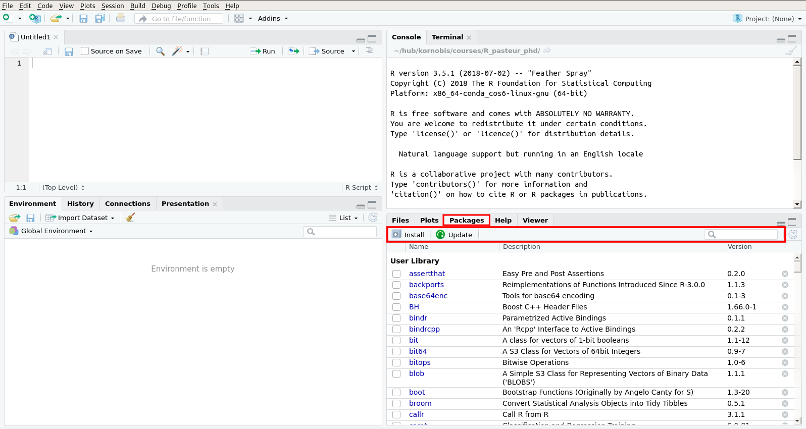
17.3.2 Installing packages using the console

To install a package, you can also simply use its name as argument to the install.packages function. For example to install the dplyr package:

install.packages("dplyr")

What can you try right now in order to avoid wasting time installing packages during the “Multivariate analysis” course?

Hint

install.packages("FactoMineR")
install.packages("factoextra")

You can also give a vector of package names to install.packages:

install.packages(c("FactoMineR", "factoextra"))

If some packages fail to install, have a look at the troubleshooting section.

17.3.3 Troubleshooting installation

If the installation fails, you may have to install other things which are not part of R, like compilers (tools that transform code into working executable programs) and development libraries (files providing more or less general functionalities that multiple programs can use).

Watch out for possible error messages during the installation process. This will give you ideas of keywords to use when searching for a solution on the internet in case something goes wrong.

If you are using Mac OSX, you might find some of the missing tools here: https://cran.rstudio.com/bin/macosx/tools/.

If you are using Linux, the information here might help: https://github.com/blaiseli/R_install_notes/blob/master/Install_Linux.md.

Sometimes, a failure to install packages may be due to incompatibilities between packages. In such a case, something you can try is to use an alternate package manager, such as Bioconductor.

17.3.4 Bioconductor

There is an effort of the bioinformatics community to provide a set of specialized R packages through it’s own system: Bioconductor (which actually uses install.packages under the hood).

Bioconductor strives to provide a set of compatible packages, and can also install R packages that are not specific to bioinformatics.

To be able to install packages via Bioconductor, you should first install the BiocManager package:

install.packages("BiocManager")

Then, you can install packages using the BiocManager::install function. For instance, to install the differential expression analysis package DESeq2:

BiocManager::install("DESeq2")

You will likely be able to use this instead of install.packages in most cases, not only for bioinformatics-specific tools.

For instance if you encountered issues installing packages for PCA you may try the following:

BiocManager::install("FactoMineR")
BiocManager::install("factoextra")

17.3.5 Using a package

Once the package of interest is installed, we should be able to use functions provided by this package.

To load all the functions of the package into your current session, you can use the function library: For example with the dplyr package:

library("dplyr")
# Then the "full_join" function from dplyr is available for the current session:
counts_WT_bis <- full_join(counts_WT_1, counts_WT_2, by = "gene_name")

Or you can use a specific function from this package using the package name and double colons (::) as prefix.

For example, if you want to use only the function full_join of the dplyr package:

counts_WT_bis <- dplyr::full_join(counts_WT_1, counts_WT_2, by = "gene_name")

18 Cheat Sheet

18.1 Number notation

• .: decimal separator in a number
• 2e3: 2 times (10 to the power of 3)
• 1L: forced integral number

18.2 Operators

• +, -, *, /: the standard mathematical operators
• %%, %/%: modulus and integer division
• x^n: x to the power of n
• log2(x), log10(x), log(x, base=n): logarithms
• <, >, <=, >=, ==, !=: comparison operators

18.3 Boolean computations

• TRUE, FALSE: literal Boolean values (without quotes)
• |, &, !: Boolean OR, AND and NOT.
• ifelse(condition, do_if_true, do_otherwise): deciding what to do depending on the Boolean condition
• is.na: test whether values are NA (== NA returns NA)

18.4 Strings

• "word": literal character strings are between quotes
• "": empty string
• paste(s1, s2, sep=s): join strings s1 and s2 using separator s (s1 and s2 can also be vectors of strings)
• "\t", "\n": special characters for tabulation and new line
• cat: human-friendly displaying of strings

18.5 Factors and formulae

• stringsAsFactors=FALSE: tell some functions to keep strings as strings
• as.factor(s): convert string s into factors
• levels(f): get or set the levels of factors f
• factor(c("a", "b"), levels=c("a", "b", "c")): factors with extra levels
• tapply(v, f, func): apply func on elements of v partitioned according to the corresponding factors in f
• formulae?

18.6 Vector creation

• c: combine values of a same type in a vector (c() creates an empty vector)
• c(a=1, b=2): create a vector with named elements
• n:m: Vector of numbers from n to m
• seq(n, m, by=i): sequence from n to m incrementing by i
• rep: repeat values
• rnorm(n, mean=m, sd=s): n random numbers from a normal distribution
• sample(v, n, replace=TRUE): random sample of n elements from vector v, with possibly multiple occurrences of an element
• vector(length=n, mode="numeric") initialize a vector with n default numeric values (0)

18.7 Repeating a computation

• replicate(n, f(x)): n values obtained by calling f(x)
• for (i in 1:n) {f(i)}: repeat a computation with i successively assuming the values from 1:n
• i <- 1; while (i <= n) {f(i); i <- i + 1}: repeat a computation while a condition is TRUE (; \(\Leftrightarrow\) new line)

18.8 Operations on vectors

• values get recycled when operating between vectors
• length(v): number of elements in v
• v[n]: get the n\(^{th}\) value in v (also works with multiple indices)
• v[n:m]: get from the n\(^{th}\) to the m\(^{th}\) value in v
• v[b], with b a vector of Booleans: get the values from v where b is TRUE
• which[b]: indices where b is TRUE
• sum(v): sum of the elements in v

18.9 Matrices

• cbind, rbind: stack vectors by columns or by rows (recycling shorter vectors and converting types if necessary)
• matrix(v, nrow=n, ncol=m): reshape vector v into an n \(\times\) m matrix
• dim: get or set number of rows and columns
• mat[n,]: get n\(^{th}\) row (several rows if length(n) > 1)
• mat[,m]: get m\(^{th}\) column (several rows if length(m) > 1)
• mat[n,m]: get value at coordinates (n, m)
• t(mat): transpose matrix mat

18.10 Lists

• list(A=v1, B=v2): list with two named elements A and B made from arbitrary values v1 and v2 (names are optional)
• names: get or set elements names
• l[[n]]: get the n\(^{th}\) element
• l$A: get the element named A

18.11 Data frames

• data.frame(A=c1, B=c2): data frame with two named columns A and B made from vectors v1 and v2 (names are optional)
• data.frame(..., stringsAsFactors=FALSE): keep strings as strings
• names, colnames: get or set column names
• rownames: get or set row names
• df[n,]: get n\(^{th}\) row (several rows if length(n) > 1) as a data frame (row names can be used instead of numbers)
• df[b,]: get rows where Boolean vector b is TRUE, as a data frame
• df$A, df[,"A"], df[,m]: get column A (or m\(^{th}\)) as a vector
• df[, c("A", "B")], df[, 1:2]: get columns A and B (or from 1 to 2) as a data frame (more than one column cannot be just a vector)
• df[n,m]: get value at row n and column m (numbers or row and column names can be used)
• df$C <- v3: change or add column C using vector v3
• merge(df1, df2, by="A"): merge data frames d1 and d2 based on column A
• rowMeans, rowSums, colMeans, colSums: quick means or sums of rows or cols (argument na.rm=TRUE to ignore missing values)

18.12 Paths, files, input / output

• getwd: Where am I?
• setwd(path): I want to be at path.
• dir.create(path): creating a directory at path
• cat(string, file=path): write string into file at path
• read.table(path): read file at path into data frame, various arguments:
  • header=TRUE: use first line as column names
  • stringsAsFactors=FALSE: keep strings as strings
  • sep="\t": column separator is tabulation
• write.table(df, file=path): write data frame df into file at path, various arguments:
  • sep="\t": column separator is tabulation

18.13 Functions

• f <- function(args) {body}: defining a function f using args in code body
• f(args): executing f using args
• function() {instr_1; instr_2}: return the value of instr_2 (; \(\Leftrightarrow\) new line)
• function() {return instr_1; instr_2}: return the value of instr_1, don’t execute instr_2

18.14 Examining, visualizing

• head, tail: first and last elements
• nrow, ncol, dim: get dimensions
• min, max, range, mean, var, sd, median, quantile, IQR, summary: descriptive statistics
• class: information about class of data
• str: structure of something
• table: easy counting
• hist: plot histogram
• barplot: plot bar plots
• boxplot: box-and-whiskers plots
• plot: versatile plotting function
• abline: straight lines on an existing plot
• par: graphical parameters (to customize your graphs)