Classification on Titanic Data set
%pylab inline
import pandas as pd
matplotlib.rcParams['figure.figsize'] = (10,6)
The data
training= pd.read_csv("data/titanic_training.csv", index_col=0)
test = pd.read_csv("data/titanic_test.csv", index_col=0)
Data description
training.head(3)
Survived : 1 means survived (remember True is 1)
Data visualisation
training.survived.value_counts().plot(kind="bar")
title("Survival (1=survived)")
grid()

training[["survived", "age"]].boxplot(by="survived")

training.pclass.value_counts().plot.barh()
title("class distribution")
grid()

Cleanup
- Remove useless features or features with lots of missing values
- drop remaining rows with at least one missing values
# many missing values
print(len(training), len(test))
ignore = ["cabin", "home.dest", "body", "embarked", "boat"]
training.drop(ignore, axis=1, inplace=True)
test.drop(ignore, axis=1, inplace=True)
training.dropna(inplace=True)
test.dropna(inplace=True)
print(len(training), len(test))
Let us replace male by 0 and female by 1
training = training.replace("male", 0).replace("female", 1)
test = test.replace("male", 0).replace("female", 1)
Find a relevant feature of interest
male_survived = len(training.query("sex==0 and survived==1"))
N_male = len(training.query("sex==0"))
male_survival_rate = male_survived / N_male * 100

female_survived = len(training.query("sex==1 and survived==1"))
N_female = len(training.query("sex==1"))
female_survival_rate = female_survived / N_female * 100

bar([0,1], [male_survival_rate, female_survival_rate ])
xticks([0,1], ['male', 'female'])
xlabel("survival rate (%)")

The training and test data
features = ["sex"]

Y = training.survived.values
X = training.loc[:, features].values

Ytest = test.survived.values
Xtest = test.loc[:,features]
Your own naive classifier
Let us predict the survival as follows:
- if it is a woman: survives
- if it is a man: does not survive
This is a simple as :
Y_pred = (Xtest.sex == 1)
Accuracy = fraction of all instance that are correctly categorized
sum(Y_pred == Ytest)/len(Y_pred)
What about a proper classifier from sklearn ?
from sklearn.linear_model import SGDClassifier
clf = SGDClassifier()
clf.fit(X, Y)
# Let us save the prediction for later
Y_pred_1 = clf.predict(Xtest)

clf.score(Xtest, Ytest)
The score is not deterministic ! See later
Stochastic Gradient Descent classifier
Stochastic Gradient Descent (SGD) is a simple yet very efficient approach to discriminative learning of linear classifiers under convex loss functions such as (linear) Support Vector Machines and Logistic Regression.
SGD has been successfully applied to large-scale and sparse machine learning problems often encountered in text classification and natural language processing.
The advantages of Stochastic Gradient Descent are:
- Efficiency.
- Ease of implementation (lots of opportunities for code tuning).
The disadvantages of Stochastic Gradient Descent include:
- SGD requires a number of hyperparameters such as the regularization parameter and the number of iterations.
- SGD is sensitive to feature scaling.
Binary classifiers
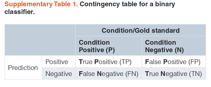
See page 17-20 from https://f1000research.com/articles/4-1030/v1 for all definitions
ROC curve
from sklearn import metrics
fpr1, tpr1, thresholds = metrics.roc_curve(Ytest, Y_pred_1, pos_label=1)
metrics.roc_auc_score(Ytest, Y_pred_1)
plot(fpr1, tpr1, "o-")
plot([0,1], [0,1], "-k")

scores = []
for this in range(20):
    clf = SGDClassifier()
    clf.fit(X, Y)
    scores.append(clf.score(Xtest, Ytest))
    prediction = clf.predict(Xtest)
    fpr, tpr, thresholds = metrics.roc_curve(Ytest, prediction, pos_label=1)
    plot(fpr, tpr, "-o")
mean(scores), std(scores)

Add more features
features = ["sex", "pclass"]

Y = training.survived.values
X = training.loc[:, features].values

Ytest = test.survived.values
Xtest = test.loc[:,features].values
subplot(2,2,1)
training.query("sex==0 and pclass==3").survived.value_counts().plot(
    kind="bar", label='male class2')
legend(); xticks([0,1], ["survived", "died"])
subplot(2,2,2)
training.query("sex==0 and pclass!=3").survived.value_counts().plot(
    kind="bar", label='male class 2/3')
legend(); xticks([0,1], ["survived", "died"])
subplot(2,2,3)
training.query("sex==1 and pclass==3").survived.value_counts().plot(
    kind="bar", label='female class3')
legend(); xticks([0,1], ["survived", "died"])
subplot(2,2,4)
training.query("sex==1 and pclass!=3").survived.value_counts().plot(
    kind="bar", label='female class 2/3')
legend();  _ = xticks([0,1], ["survived", "died"])

clf = SGDClassifier()
clf.fit(X, Y)
clf.score(Xtest, Ytest)
Note that it is stochastic so sometimes 2 features is worst than 1 but on average it is better
scores = []
for this in range(20):
    clf = SGDClassifier().fit(X, Y)
    scores.append(clf.score(Xtest, Ytest))
    prediction = clf.predict(Xtest)
    fpr, tpr, thresholds = metrics.roc_curve(Ytest, prediction, pos_label=1)
    plot(fpr, tpr, "-o")
mean(scores), std(scores)

What about KNearestNeigbors classifier ?
features = ["sex"]
Y = training.survived.values
X = training.loc[:, features].values
Ytest = test.survived.values
Xtest = test.loc[:,features].values
from sklearn.neighbors import KNeighborsClassifier
clf = KNeighborsClassifier()
clf.fit(X, Y)
clf.score(Xtest, Ytest)
features = ["sex", "pclass",]
Y = training.survived.values
X = training.loc[:, features].values
Ytest = test.survived.values
Xtest = test.loc[:,features].values
from sklearn.neighbors import KNeighborsClassifier
clf = KNeighborsClassifier()
clf.fit(X, Y)
clf.score(Xtest, Ytest)
Decision Trees
Decision Trees (DTs) are a non-parametric supervised learning method used for classification and regression. The goal is to create a model that predicts the value of a target variable by learning simple decision rules inferred from the data features.
some advantages:
- simple to understand (see later)
- low cost (log)
- handle categorical and numerical data (less data preparation)
some drawbacks:
- can be unstable. small variation may lead to different results
- may perform overfitting (over complex tree)
from sklearn import tree
clf = tree.DecisionTreeClassifier()
clf.fit(X, Y)
clf.score(Xtest, Ytest)
import pydotplus
dot_data = tree.export_graphviz(clf, out_file=None)
graph = pydotplus.graph_from_dot_data(dot_data)
dot_data = tree.export_graphviz(clf, out_file=None,
                         feature_names=features,
                         class_names=["survived", "died"],
                         filled=True, rounded=True,  special_characters=True)
graph = pydotplus.graph_from_dot_data(dot_data)
from IPython.display import Image
Image(graph.create_png())

RandomForest
Random forests are an ensemble learning method for classification (and regression) that operate by constructing a multitude of decision trees at training time and outputting the class that is the mode of the classes output by individual trees.
-- wikipedia
From sklearn website:
In random forests each tree in the ensemble is built from a sample drawn with replacement (i.e., a bootstrap sample) from the training set.
In addition, when splitting a node during the construction of the tree, the split that is chosen is no longer the best split among all features.
Instead, the split that is picked is the best split among a random subset of the features. As a result of this randomness, the bias of the forest usually slightly increases (with respect to the bias of a single non-random tree) but, due to averaging, its variance also decreases, usually more than compensating for the increase in bias, hence yielding an overall better model.
from sklearn.ensemble import RandomForestClassifier

clf = RandomForestClassifier(n_estimators=5)
clf.fit(X, Y)
clf.score(Xtest, Ytest)
Neural network
from sklearn.neural_network import MLPClassifier
clf = MLPClassifier(solver='lbfgs', alpha=1e-5,
                    hidden_layer_sizes=(10, 1), random_state=1)
_ = clf.fit(X, Y)
clf.score(Xtest, Ytest)
Cross validation for binary classifiers
training.head(3)
features = ["sex", "class"]
Y = training.survived.values
X = training.loc[:, features].values
Ytest = test.survived.values
Xtest = test.loc[:,features].values
from sklearn.model_selection import cross_val_score
clf1 = tree.DecisionTreeClassifier()
clf2 = SGDClassifier()
clf3 = KNeighborsClassifier()
clf4 = RandomForestClassifier(n_estimators=10)

scores1 = cross_val_score(clf1, X, Y, cv=5)
scores2 = cross_val_score(clf2, X, Y, cv=5)
scores3 = cross_val_score(clf3, X, Y, cv=5)
scores4 = cross_val_score(clf4, X, Y, cv=5)


yerr = [std(this) for this in [scores1, scores2, scores3, scores4]]
mus = [mean(this) for this in [scores1, scores2, scores3, scores4]]
errorbar([0,1,2,3], mus, yerr=yerr, xerr=0.1, fmt="o")
ylim([0.5,1])
_ = xticks([0,1,2,3], ["tree", "sgd", "kn", "RF"], rotation=0, fontsize=40)
print(mus)

Summary
- Select the relevant features
Remove or impute missing data sets
choose a classifier. We have seen:
- KNeighbor
- DecisionTree
- StochasticGradient
but there are many more. See sklearn website
This section was used to create the training and test set from the whole data
from sklearn.utils import shuffle
df = pd.read_csv("data/titanic3.csv")
df = shuffle(df)
training = df.ix[df.index[0:916]]
test = df.ix[df.index[916:]]
training.to_csv("data/titanic_training.csv")
test.to_csv("data/titanic_test.csv")
pd.read_csv("data/titanic_training.csv", index_col=0)