
Institut Pasteur, Paris, 20-31 March 2017
Motivation
- Python is a general-purpose language. It was not designed for scientific computing.
- NumPy is the core tools for performant numerical computing with Python. It is used by many other scientific libraries including SciPy, Pandas, matplotlib.
Installation
(in terminal)
conda install numpy
Convention
import numpy as np
Arrays
an array is like a sequence but contains a homogeneous collections of items (e.g. all integers)
import numpy as np
x = np.array([1, 2, 3])
x
NB1:
x is an instance of the object numpy.ndarray. The constructor takes as argument a sequence. Here we provided a list hence the ([ ]) syntax.
NB2: Following the previous nota bene about the syntax we have:
a = np.array(1, 2, 3, 4)    # WRONG
a = np.array([1, 2, 3, 4])  # RIGHT
NumPy provides fast and memory efficient data structures
Pure Python
l = range(1000000)
%time sum(l)
Numpy
x = np.array(l)
%time x.sum()
About 15 times faster
Another example:
How would you compute $\sum X_i^2$ given $X$ is a Python list ?
l = range(1000000)
%time sum([x**2 for x in l])
x = np.array(l)
%time (x**2).sum()
!!! about 70-80 times faster
Create N-D arrays
1-D array
x = np.array([1, 2, 10, 2, 1 ])
x.shape
len(x)
Indexing follows the same syntax as with Python sequences.
x[2]
x.ndim
2-D arrays
np.array([[1,2], [3,4]])
Here is a naive way to build a 2D matrix with values going from 1 to 12. Later, we will use the arange function + reshape method
n1 = [1, 2, 3]
n2 = [4, 5, 6]
n3 = [7, 8, 9]
n4 = [10, 11, 12]
m = np.array([n1, n2, n3, n4])
m.ndim
m.shape
len(m)
Indexing: LC convention (Line / Column)
For a 5x5 matrix, the indexing works as follows
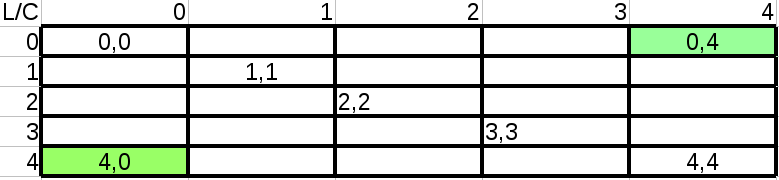
m
# To get 11, last row, second column:
m[3,1]
#equivalent but a bit slower:
m[3][1]
4-D arrays ? why not ?
Given a cubic volume of air, we decompose it in a 2x2x2 smaller cubes. In each small cube, we measure 3 variables: eg, pressure, temperature...
c1 = [1,2,3]; c2 = [1,2,3]; c3 = [1,2,3]; c4 = [1,2,3];
c5 = [1,2,3]; c6 = [1,2,3]; c7 = [1,2,3]; c8 = [1,2,3];
x = np.array(
    [                   # first dimension (2 slices)
        [               # second dimension (2 rows)
            [           # third dimension (2 columns)
                c1, c2
            ],
            [
                c3, c4
            ]
        ],
        [
            [
                c5, c6
            ],
            [
                c7, c8
            ]
        ]
    ])
x.shape
Functions to create arrays
The previous 4D example was not created by hand but based on:
The ones function
np.ones((2, 2, 2, 3))
# a 2D example
np.ones((4, 2))
The arange function
Evenly spaced values within a given interval based on a step
np.arange(1, 10) # not that the end is exclusive and the step is 1 by default
np.arange(0, 10, step=2)
# Remember how we created to first 2D example array ?
# here is the proper way with arange and reshape
np.arange(12).reshape(4,3)
the linspace function
Evenly spaced values within a given interval based on a number of points
np.linspace(0, 1, 10)
ones, zeros, diag, eye, empty
np.diag((5,5,1,1))
np.ones((2,2))
np.zeros((2,2))
np.eye(3)
Random values
Python language has its own random module but numpy has more functionalities.
# uniform random values between 0 and 1
np.random.rand()
# normal distribution. Note the **n** after rand
np.random.randn()
# array of normally distributed values
np.random.normal(size=10)
Array creation
- Create a 4x4 matrix with 2's on the diagonal. What about a 100x100 matrix ?
- Create a matrix 5x5 with random number uniformly distributed
- Creata a 1D array of 1000 points normally distributed. Compute the mean and standard deviation.
- Same question for a uniform distribution.
- can you compute the maximum and miminum of the previously created arrays. Does it make sense ?
- Create these matrices:
and1 0 0 0 0 0 1 0 0 0 0 0 5 0 0 0 0 0 1 0 0 0 0 0 10 1 1 1 1 1 0 1 1 1 1 1 -4 1 1 1 1 1 0 1 1 1 1 1 0
Hints and solutions
# 1 -
x = np.diag([2,2,2,2]);
x = np.diag([2]*100);
# 2 -
x = np.random.normal(size=25).reshape(5,5)
# 3 -
x = np.random.normal(size=1000)
x.mean()
x.std()
# 4 - for uniform distribution, replace 'normal' by 'uniform'
# 5 -
x.min()
x.max()
# takes the min/max of U should give [0,1] and on N should give
# -2, +2 but random so may change. does it make sense -> yes
# 6 -
A = np.diag([1]*5); A[2,2]=5
B = np.ones((5,5)) - A
data types
x = np.array([1, 2, 3])
x.dtype
x = np.array([1., 2, 3.5])
x.dtype
x = np.array([1, 2, 3], dtype=float)
x.dtype
x = np.array([1, 2, 3])
x = x.astype(float)
x
np.array([1.0, 1, "oups"])
Basic indexing and slicing
- Create an array that goes from 0 to 9 (included)
Using slicing and indexing:
- Select only odd values
- Select only even values
- Select last two values only
- Select all values except first 2
Note that the syntax is the same as in pure Python slicing and indexing
Solutions
data = np.arange(10)
# you may use pure python and cast to array:
data = np.array(range(10))
print("even: {}".format(data[::2]))
print("odd: {}".format(data[1::2]))
print("last two : {}".format(data[-2:]))
print("from pos 1: {}".format(data[2:]))
Example in 2D
Syntax. First index is for rows and second for columns:
    Matrix[0, :]
    Matrix[:, :]
    Matrix[:, 0]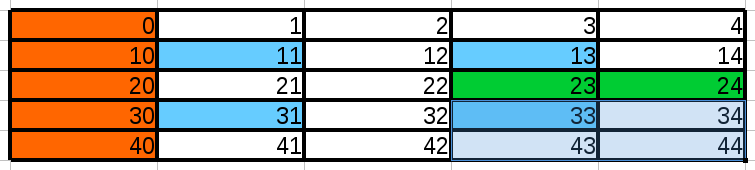
Create the array shown above. Then, with slicing and indexing,
- extract first row,
- extract first column (orange cells)
- extract even values only, odd values only
- extract the 4 blue cells
- extract the 2 green cells
- extract the 2x2 sub-matrix in bottom right corner
Solutions
# blue cells
x = np.arange(5)
M = np.array([x, x+10, x+20, x+30, x+40])
# first row:
M[0,:]
# first colum,n
M[:,0]
# even values
M[:,::2]
# odd values
M[:, 1::2]
# sub corner:
M[-2:, -2:]
# green cells:
M[2, 2:]
# blue cells:
M[1::2, 1::2]
Copies and views
Like in Python, we are manipulating objects. So be careful with the references
a = np.array([1,2,3,4,5])
b = a[:]
a[2] = 30
b
b[-2:] = 0
b
a
copies
a = np.array([1,2,3])
b = a.copy()
b[1] = 100
b
a
Fancy indexing
As we have seen before, standard Python slicing and indexing works on NumpPy array. Yet, NumPy provides more indexing, which can be performed with boolean or integer arrays, also called masked
Indexing with boolean masks
Boolean mask is a very powerful feature in NumPy. It can be used to index an array, and assign new values to a sub-array. Note also that it creates copies not views
data = np.arange(16)
data
Find all multiple of 7
(data % 7 == 0)
mask = (data % 7 == 0)
data[mask]
# Replaces values:
data[mask] = -100
data
Indexing with an array of integers
X = np.array([-1, 2, -3, -4, -5, 10, 20])
indices = [0, 1, 2, 3]
X[indices]
Indices are nice if you have uneven selection and you know what you want before hand
indices = [0,4]
X[indices]
Of course in the first example, we could have been smarter with just a mask:
X[X<0]
Fancy indexing
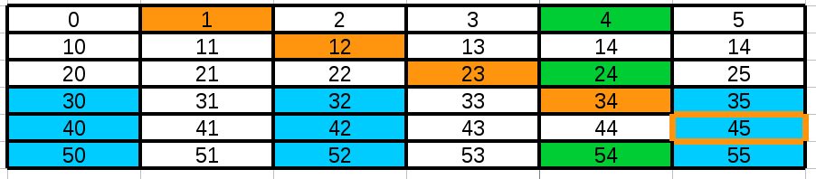
Create the array above and extract the following data sets:
- the 9 blue cells
- the 5 orange cells
- the green cells
Solutions
x = np.arange(6)
M = np.array([x, x+10, x+20, x+30, x+40, x+50])
M
# Creation using tiles
M = np.tile(range(6), (6, 1))
for i in range(6):
    M[i,:] += i*10
M
# orange:
M[(0,1,2,3,4), (1,2,3,4,5)]
# blue:
M[3:, [0,2,5]]
# green:
M[np.array([1, 0,1,0,0,1], dtype=bool),4]
# green:
M[np.array([True, False,True,False,False,True]),4]
- Create a range from -5 to 5 (included)
- With a mask, find the positive values and replace them with +1
- With a mask, find the negative values and replace them with -1
Solutions
M = np.arange(-5,6)
M[M<0]
M[M>0]
Numerical operations
A = np.array([[4, 7],
              [2, 6]])

B = np.array([[0.6, -0.7],
              [-0.2, 0.4]])
A + B
C = B.copy()
C *= 2
B         # unchanged because we did a copy !
# elementwise product
A * B
# matrix product
A.dot(B)
A.dot(B).round()
Comparisons
a = np.array([1,2,3,4])
b = np.array([1,2,3,100])
a == b
a > b
array-wise comparison
# method1
np.array_equal(a, b)
# method2
np.all(a==b)
Logical operations
a = np.array([1,1,0,0])
b = np.array([1,1,0,1])
OR / AND operations
np.logical_or(a,b)
Comparison and logical operations return array of boolean type, so can be used as mask to select a sub set
Exercices
a = [1,1,0,1,1]
b = [0,1,0,1,0]
c = [1,2,3,4,5]
- In pure Python, check that a*b does not work.
- In pure Python, compute the a*b on an element-wise basis For instance [1,2][2,3] should give [2,6]. Apply to **ab**
- In pure Python, compute the logical AND of a with respect to b (element-wise)
- Same question: compute a*b in Pure Numpy
- Guess (without typing the code) the output of
np.array([True, 1, 2]) + np.array([3, 4, False])- Guess the output of
np.array([[1,2], [3,4], [5,6]]).shape
Solutions
a = [1,1,0,1,1]
b = [0,1,0,1,0]
c = [1,2,3,4,5]
# 1.
# 2.
[x*y for x,y in zip(a,b)]
# 3.
a and b # we get ones and zeros, but no boolean values
[x and y for x,y in zip(a,b)]
[bool(x and y) for x,y in zip(a,b)]
# 4. in numpy:
np.logical_and(a,b)
# 5.
# [4,5,2]
# 6.
# the dimension of the matrix
(3, 2)
Some linear algebra ?
from numpy import linalg
\begin{equation} A * A^{-1} = I \end{equation}
A = np.array([[4, 7],
              [2, 6]])
B = linalg.inv(A)
B
A.dot(B).round()
Reductions (function applied on 1 axis)
x = np.array([1, 2, 3, 4, -1, -2, -3, -4])
x.sum()
x.min()
x.max()
# Position of the max
x.argmax()
Reduction in higher dimensions
A = np.array([
    [1,10,1],
    [2,8,3]
])
A.sum()
What about sum along the first axis (Line)
What about sum along the second axis (Column)
# Compute the sum along the axis 0 (rows). You reduce the row,
# so in this example you should end up with 3 values
A.sum(axis=0)
# Here, we sum along axis 1 so we should get the sum for each line.
A.sum(axis=1)
Reductions
- Create a 1,000,000 long vector (whatever distribution) but with positives and negatives values.
- Write 3 functions to get the max using
- numpy max method,
- pure Python max function,
- a loop searching for the max (keeping track of the max). Compare the computation times
- Create a 2x3 matrix with random values (negative/positive). Experiments with the mean, max, argmin, argmax absolute, std.
- On the previous example, check that the transpose() method is equivalent to reshape(3,2)
Solutions
#1.
X = np.random.randn(1000000)

#2.
def max_numpy(X):
    return np.max(X)
def max_python(X):
    return max(X)
def max_list(X):
    M = -1e6
    for this in X:
        if this > M:
            M = this
%timeit max_numpy(X)
%timeit max_python(X)
%timeit max_list(X)
# 3.
X = np.random.rand(6).reshape(3,2)
X.mean(axis=0)
Iterations
X = np.random.normal(size=12).reshape(6,2)
X
for row in X:
    if row.sum() > 0 :
        print(row)
for item in X.flat:
    if item >1:
        print(item)
Iterations
- Given an array 6x2 of random numbers normally distributed, loop over the row and print the row when there is at least one positive value
- Given the same 6x2 matrix, loop over the rows, and print the index of the row when there is at least one positive value
solutions
np.random.seed(15)
m = np.random.randn(12).reshape(6,2)
print(m)
print("-------*---------")
for row in m:
    if sum(row>0) >0:
        print(row)
print("-------*---------")
for i,row in enumerate(m):
    if sum(row>0) > 0:
        print(i)
inf and nan
res = np.sqrt(-1)
res
np.isnan(res)
import sys
sys.float_info.max
res = np.array([1e308,1e300]) * 10
res
Resizing
a = np.diag([1,2,3,4])
# Can be used to add a column or a row
a.resize((5,4))
a
Restriction: no reference permitted
Sorting
X = np.array([5,1,10,2,7,8])
X.sort() # inplace
X
X = np.array([5,1,10,2,7,8])
np.sort(X)
X = np.array([5,1,10,2,7,8])
X.argsort()
Loading data
Numpy has its own reader of tabulated data sets (e.g. genfromtext)
data = np.genfromtxt("data/numpy.csv", delimiter=",")
data[:,1]
However, we will use pandas read_csv function that is far better
CSV that genfromtext does not handle:
- strings that contains comma (see data/chembl.csv)
- mix of integers and strings (see data/brain_size.csv)
vstack and hstack (will be used in other notebooks)
a = np.array([1, 2, 3])
b = np.array([4, 5, 6])
np.vstack([a, b])
# equivalent of the + operator with list
np.hstack([a, b])
Summary
For scientific computation with large data sets, use NumPy what you should keep in mind:
- How to create arrays with : array, arange, ones, diag, zeros, ...
- Know the shape and dimensions
- Perform slicing and indexing at least on 2D arrays
- How to use operators. Keep in mind that * operator is an element-wise operation.
- Reduction operations: min,max, argmax, argmin, std, var, mean, absolute
- Maths operators: abs, add, arccos,round, floor, cum, cumsum
- ordering, sorting: argmax, sort, argsort
To go further:
- Broadcasting: operations on array with differen sizes
- splitting arrays
- check out some other functions: convolve, correlate, corrcoef, cov
References: NumPy documentation and Scipy Lectures Notes