 TC, BN, JBM, AZ
Institut Pasteur, Paris, 20-31 March 2017
Definition
The field of machine learning is concerned with the question of how to construct computer programs that automatically improve with experience.
Machine learning is not only about learning from data but also predicting
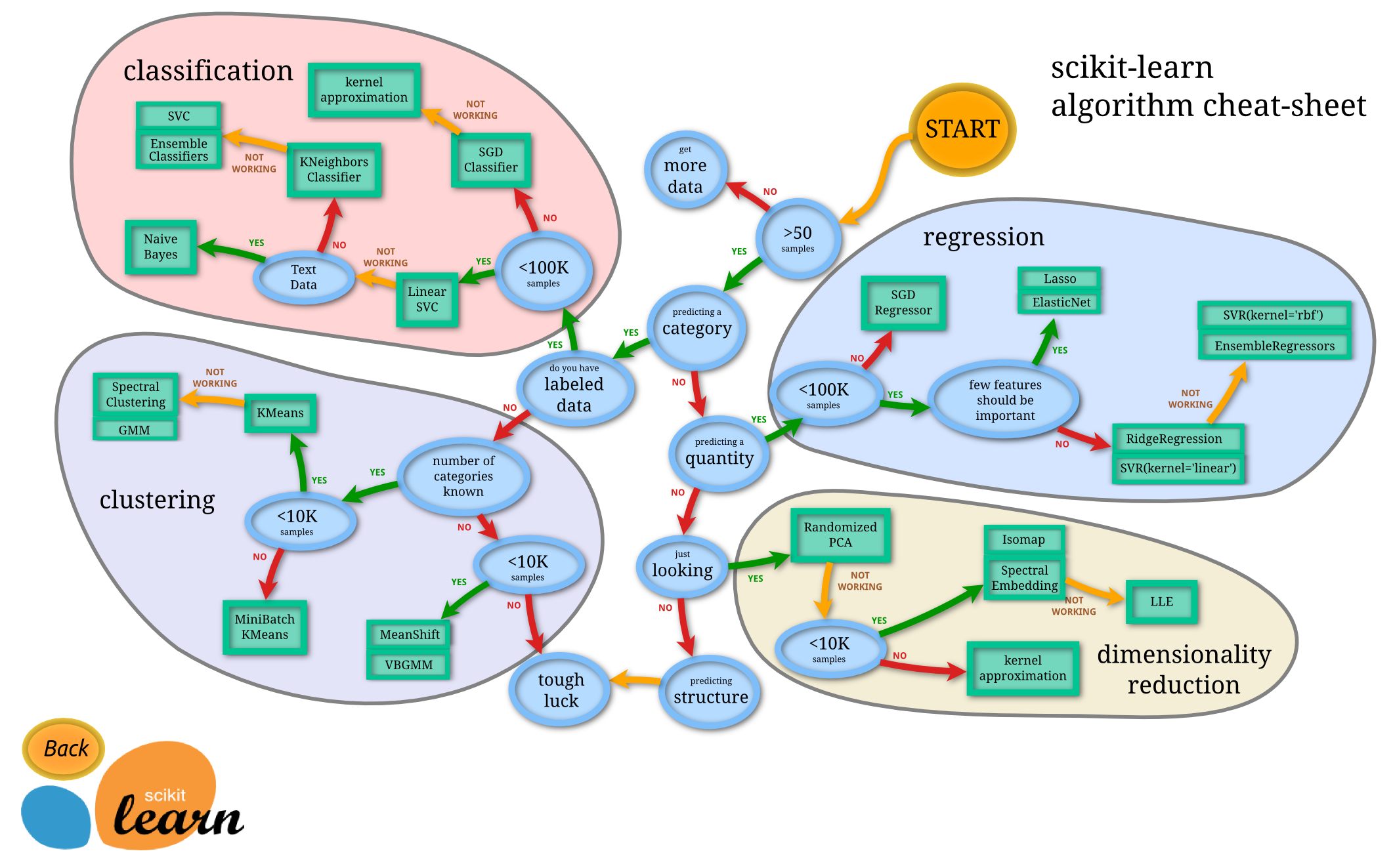
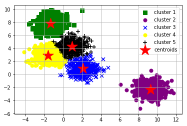
Goal of unsupervised methods: find hidden patterns in a dataset from unlabeled data.
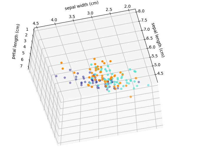
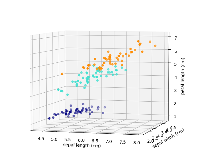
For example: clustering of cancer cell lines based on their gene expression profile (expected to group by their respective tissue-of-origin); identification of the number of different species based on their phenotypes; dimensionality reduction...
Goal of supervised methods: inferring a function from labeled data.
- regression: we observe a response or outcome variable (e.g., drug response) and a set of features/variables (e.g., molecular biomarkers like somatic mutations). The goal is then to predict the response of a new drug using the features.
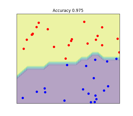
- classification: samples that belong to two more classes. From already labelled data, how to predict the class of unlabelled data (digit recognition).
Introductory example: linear regression
Linear Regression is an approach for modelling the relation between a scalar dependent variable $Y$ and one or more explanatory variables $X$.
Usually, the measurements are noisy; an additional disturbance term or error variable is present. If we denote $\epsilon$ the error variable, the linear model can be written as
\begin{equation} \rm{Y} = \beta_0 + \beta_1 \; \rm{X} + \epsilon, \end{equation}
where $\beta_1$ is a parameter also called effects or regression coefficients that needs to be estimated. The parameter $\beta_0$ is the intercept.
We can of course have several dimensions (explanatory variables)
\begin{equation} \rm{Y} = \beta_0 + \beta_1 \; \rm{X}_{1} + \beta_2 \; \rm{X}_{2} + \epsilon_i, \end{equation}
Linear equations
import toolkit
subplot(1,2,1); toolkit.figure_intro_regression()
subplot(1,2,2); toolkit.figure_intro_poly()

Linear equation: Since terms of linear equations cannot contain products of distinct or equal variables, nor any power (other than 1) or other function of a variable, equations involving terms such as $xy$, $x^2$, $y^{1/3}$, and $\sin(x)$ are nonlinear.
Fitting
Linear regression fits a linear model with coefficients $\beta = (\beta_1, \dots \beta_p)$ to minimize the residual sum of squares between the observation $Y$, and the responses predicted by the linear model
\begin{equation} min_\beta || X \beta - Y ||^2_2 \end{equation}
We can try manually but of course this would need to be automatized
Guess the best intercept and coefficient of regression
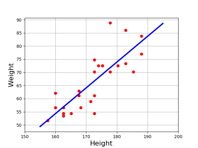
Using the following X, Y data sets, guess the intercept and coefficient of regression using visual introspection and plotting. !! No minimization !! We can assume that
$Y = intercept + coefficient * X $
df = pd.read_csv("data/weights.csv")
X, Y = df.height.values, df.weight.values
Intercept -105 and a slope of 1 seems a good choice
import pandas as pd
df = pd.read_csv("data/weights.csv")
X, Y = df.height.values, df.weight.values
plot(X, Y, "o")
plot(X, -105 + X, lw=4, alpha=0.5)
grid()

Build a data set (linear)
Write a function that takes as input 3 parameters: N, sigma and a seed The function returns two vectors X and Y of length N. The X vector is a 1D numpy array with evenly spaces values between -5 and 5. Y is a 1D numpy array such that
$Y = 2 + X + \mathcal{N}(0, \sigma)$,
where $\mathcal{N}(0, \sigma)$ is a gaussian noise (normal). Set this default values: N=10, seed=1, sigma=0.5
hints: for the gaussian distribution, search in numpy.random --
def linear_equation(N=10, sigma=0.5, seed=1):
    np.random.seed(seed)
    X = np.linspace(-5, 5, N)
    Y = 2 + X + sigma * np.random.normal(size=N)
    return X, Y
Fitting a linear model
Let us create the X and Y data (need to reshape the X data in a 1-column shape)
X, Y = linear_equation()
X = X.reshape(-1, 1)
Now let us create a LinearRegression object from scikit-learn
from sklearn import linear_model
estimator = linear_model.LinearRegression()
And fit the data
model = estimator.fit(X, Y)
The fitted model
Let us explore the object (searching for attributes) and evaluate the quality of predictions
First, what is the coefficient of regression:
model.coef_
And intercept ($\beta_0$):
model.intercept_
Visual validation
plot(X, Y, "o")
plot(X, model.intercept_ + model.coef_ * X, lw=4, alpha=0.5)
grid()

Guess the best intercept and coefficient of regression
Using scikit learn and the following data
df = pd.read_csv("data/weights.csv")
X, Y = df.height.values, df.weight.values
- Fit a linear model. Find the intercept and coefficient of regression.
- Plot the data and corresponding fitted linear regression
df = pd.read_csv("data/weights.csv")
X, Y = df.height.values, df.weight.values
X = X.reshape(-1,1)
estimator = linear_model.LinearRegression()
model = estimator.fit(X, Y)
plot(X, Y, "o")
plot(X, model.intercept_ + model.coef_*X)
print("Intercept: {}; coeff={}".format(model.intercept_, model.coef_))

Prediction
The predict method computes the model given X, so it returns \begin{equation} Y_{\rm{prediction}} = \beta_0 + \beta_1 X \end{equation}
Y_pred = model.predict(X)
You can check that the manual computation is the same:
Y_pred - (model.intercept_ + model.coef_ *X).T
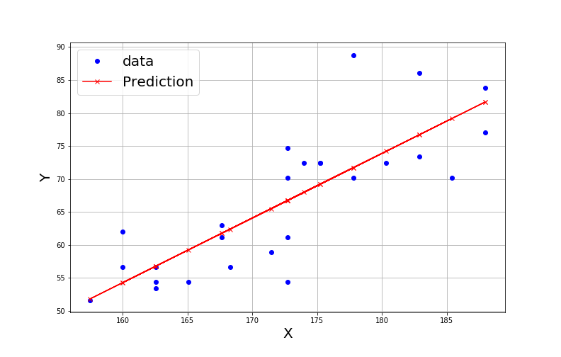
Redo the previous exercice with the **predict** method
Using scikit learn and the following data
df = pd.read_csv("data/weights.csv")
X, Y = df.height.values, df.weight.values
- Fit a linear model. Find the intercept and coefficient of regression.
- Create the following plot with the data and linear regression
# Create the data
df = pd.read_csv("data/weights.csv")
X, Y = df.height.values, df.weight.values
X = X.reshape(-1,1)

# fitting and prediction
estimator = linear_model.LinearRegression()
model = estimator.fit(X, Y)
Y_pred = model.predict(X)

# plotting
plot(X, Y, "bo", label="data")
plot(X, Y_pred, "xr-", label="Prediction")
xlabel("X", fontsize=20)
ylabel("Y", fontsize=20)
grid()
legend(fontsize=20)
print("Intercept: {}; coeff={}".format(model.intercept_, model.coef_))

Coefficient of determination
The score() function from the LinearRegression class returns the coefficient of determination, denoted $R^2$.
$R^2$ (R squared) is a statistic that will give some information about the goodness of fit of a model. In regression, the $R^2$ coefficient of determination is a statistical measure of how well the regression line approximates the real data points.
Another way to formulate $R^2$: metric that indicates the proportion of the variance in the dependent variable that is predictable from the independent variable
The coefficient $R^2$ is defined as $\left(1 - \frac{U}{V}\right)$, where $U$ is the regression sum of squares $\sum\left(Y_{true} - Y_{pred}\right) ^ 2$ and $V$ is the residual sum of squares $\sum \left(Y_{true} - \overline{Y_{true}} \right)^2$.
Best possible score is 1.0 and it can be negative (because the model can be arbitrarily worse).
A constant model that always predicts the expected value of $Y$, disregarding the input features, would get a $R^2$ score of 0.0.
Scoring function
- Write your own scoring function that computes the coefficient of determination that is: given two vectors X and Y, return 1 - U/V (see previous slide)
- Write your own scoring function that computes the pearson coefficient of correlation (hint: use numpy for pearson)
- What is the relation between R^2 and the pearson coefficient on a simple example ?
def determination(Y_true, Y_pred):
    # Same function as LinearRegression.score()
    U = ((Y_true-Y_pred)**2).sum()
    V = ((Y_true-Y_true.mean()) **2).sum()
    R2 = (1-U/V)
    return R2

def pearson(Y_true, Y_pred):
    return np.corrcoef(Y_true, Y_pred)[0,1]

Y_pred = model.predict(X)

print(determination(Y, Y_pred))
print(pearson(Y, Y_pred))

determination(np.array([1,2,3,4]), np.array([1,1,3,5]))
# example of negative value
determination(np.array([1,2,3,4,5,7,1,2,3,4,5,7]),
              np.array([0,1,0,1,0,1,0,1,0,1,0,1]))
Scoring function
model.score(X, Y)
Summary of the LinearRegression
estimator = linear_model.LinearRegression()
model = estimator.fit(X, Y)
Y_pred = model.predict(X)
score = model.score(X, Y)
# plotting
plot(X, Y, "o", label="Data")
plot(X, Y_pred, label="Prediction", lw=4, alpha=0.5)
xlabel("X", fontsize=20); ylabel("Y", fontsize=20)
grid(); title("$R^2$ = {:.4f}".format(score), fontsize=20)

Effect of the noise and pertinence of $R^2$
Noisy data and $R^2$ significance
- Write a function that takes 2 inputs: N and sigma. The parameter N is the length of the data and sigma the normal distribution sigma parameter.
- The function generates random data (re-use the function linear_equation from previous slides that generates X and Y random data where $Y = 2 + X + \mathcal{N}(0, \sigma)$. The input parameters N and sigma are the input parameter of this linear_equation function.
- Then, the function fits a linear model on the data based on LinearRegression class.
Finally, the function returns the coefficient of determination
based on the function you have created, call the function 1000 times with $\sigma = 0.5$ and 1000 times with $\sigma = 1000$. Save the results in two variables (e.g. scores1 and scores2). Plots the histograms of scores1 and scores2 in the same figure.
def get_score(N=10, sigma=0.5, show=True):
    import random
    X, Y = linear_equation(N=N, sigma=sigma,
                           seed=np.random.randint(100000))
    X = X.reshape(-1,1)
    estimator = linear_model.LinearRegression()
    model = estimator.fit(X, Y)
    return model.score(X, Y)
scores = [get_score(N=20, sigma=0.5, show=False) for x in range(1000)]
scores_noise = [get_score(N=20, sigma=100, show=False) for x in range(1000)]
bins = linspace(0,1,100)
_ = hist(scores, ec="k", alpha=0.5, bins=bins)
_ = hist(scores_noise, ec="k", alpha=0.5, bins=bins)

Polynomial function
Write a polynomial function
- Write a function that returns X and Y where $Y = 1 + X - X^2 + \epsilon$ and X is an evenly spaced vector from -5 to 5 with N points
- Parameter 1: N defaults to 10
- Parameter 2: sigma used to define $\epsilon$. sigma is the parameter used by the Gaussian distributed noise centered around a mean of 0.
- Parameter 3: a seed ( use np.random.seed )
- The function returns X and Y
Final functions is 5-lines long not more
def poly2_func(N=10, noise=3, seed=11):
    np.random.seed(seed)
    X = np.linspace(-5, 5, N)
    Y = 1 + X - X**2 + noise * np.random.normal(size=N)
    return X, Y
X, Y = poly2_func()
X = X.reshape(-1,1)

#plotting
plot(X, Y, "o")
plot(X, 1 + X - X**2)

fitting a polynomial function with sklearn
X, Y = poly2_func()
X = X.reshape(-1,1)
Obviously, fitting the linear model on this polynomial data does not work.
from sklearn import linear_model
estimator = linear_model.LinearRegression()
model = estimator.fit(X,  Y)
model.coef_
model.intercept_
plot(X, Y, "o")
plot(X, model.coef_[0] * X + model.intercept_)

model.score(X, Y)
PolynomialFeatures
from sklearn.preprocessing import PolynomialFeatures
from sklearn.pipeline import make_pipeline
degree = 2
model = make_pipeline(PolynomialFeatures(degree),
                      linear_model.LinearRegression())
_ = model.fit(X, Y)
model.score(X, Y)
plot(X, model.predict(X))
plot(X, Y, "o")

Exercice
Using the code from the previous slides,
- Create X, Y where Y is the polynomial $1 + X -X^2 +\epsilon$ reusing poly2_func function.
- Fit the data with a PolynomialFeatures assuming we know we have 2 degrees
- plot Y versus X and Y_predicted versus X (same as before)
- Now, we want to predict new data. Create a new X vector, call it Xnew and set it to [6,7,8]. Predict the Ynew values and plot Ynew versus Xnew on top of the previous plot. Does it look like a good prediction ?
# data
X, Y = poly2_func()
X = X.reshape(-1,1)
# fit
degree = 2
model = make_pipeline(PolynomialFeatures(degree),
                      linear_model.LinearRegression())
_ = model.fit(X, Y)

plot(X, model.predict(X))
# new predictions
newX = np.array([6,7,8]).reshape(-1,1)
prediction = model.predict(newX)
plot(X, Y, "o")
plot(newX, prediction, "or")

Overfitting
def plot_overfit(ws):
    print(ws)
    model = make_pipeline(PolynomialFeatures(ws),
                      linear_model.LinearRegression())
    _ = model.fit(X, Y)
    score = model.score(X.reshape(-1,1), Y)
    prediction = model.predict(X)
    plot(X, prediction, "x-")
    plot(X, Y, "o")
plot_overfit(10)

Overfitting
You can always fit the data with complex model but prediction is poor
for degree in range(1,11):
    model = make_pipeline(PolynomialFeatures(degree),
                          linear_model.LinearRegression())
    _ = model.fit(X, Y)
    score = model.score(X.reshape(-1,1), Y)
    plot(degree, score, "ob")
ylim([0.8,1])

Overfitting = bad prediction
model = make_pipeline(PolynomialFeatures(3),
                      linear_model.LinearRegression())
_ = model.fit(X, Y)

plot(X, Y, "o", label="data", markersize=12)

newX = linspace(-10,10, 15).reshape(-1,1)
plot(newX, 1 + newX - newX*newX, "g--", label="True")
plot(newX, model.predict(newX), "or-", label="Predicted")
ylim([-100,80]); legend(fontsize=20)

Summary
- We have seen how to fit a linear model using LinearRegression
- We have seen how to fit a Polynomial model using PolymialRegression
- The procedure follows those steps
- Get some data X / Y (we have seen univariate data but multivariate would work as well)
- Find a good estimator (e.g. LinearRegression)
- Create an instance of the estimator
- Fit the data to get a model using X as the input
- Predict response given new input data.
- We emphasize the danger of overfitting